WENSHAN ZHENG, SHIJIE ZHAO, YEHANG YIN, HUIDAN ZHANG, DAVID M. NEEDHAM, ETHAN D. EVANS, CHENGZHEN L. DAI, PETER J. LU, ERIC J. ALM, and DAVID A. WEITZ
SCIENCE 3 Jun 2022 Vol 376,Issue 6597
Strain specific single-cell sequencing
Single-cell methods are the state of the art in biological research. Zheng et al. developed a high-throughput technique called Microbe-seq designed to analyze single bacterial cells from a microbiota. Microbe-seq uses microfluidics to separate individual bacterial cells within droplets and then extract, amplify, and barcode their DNA, which is then subject to pooled Illumina sequencing. The technique was tested by sequencing multiple human fecal samples to generate barcoded reads for thousands of single amplified genomes (SAGs) per sample. Pooling the SAGs corresponding to the same bacterial species allowed consensus assemblies of these genomes to provide insights into strain-level diversity and revealed a phage association and the limits on horizontal gene-transfer events between strains.
Structured Abstract
INTRODUCTION
The human gut microbiome is a complex ecosystem specific to each individual that comprises hundreds of microbial species. Different strains of the same species can impact health disparately in important ways, such as through antibiotic resistance and host-microbiome interactions. Consequently, consideration of microbes only at the species level without identifying their strains obscures important distinctions. The strain-level genomic structure of the gut microbiome has yet to be elucidated fully, even within a single person. Shotgun metagenomics broadly surveys the genomic content of microbial communities but in general cannot capture strain-level variations. Conversely, culture-based approaches and titer plate-based single-cell sequencing can yield strain-resolved genomes, but access only a limited number of microbial strains.
RATIONALE
We develop and validate Microbe-seq—a high-throughput single-cell sequencing method with strain resolution—and apply it to the human gut microbiome. Using an integrated microfluidic workflow, we encapsulate tens of thousands of microbes individually into droplets. Within each droplet, we lyse the microbe, perform whole-genome amplification, and tag the DNA with droplet-specific barcodes; we then pool the DNA from all droplets and sequence.
In mammalian systems—the focus of most single-cell studies—high-quality reference genomes are available for the small number of species under investigation; by contrast, in complex communities of 100 or more microbial species—such as the human gut microbiome—reference genomes are a priori unknown. Therefore, we develop a generalizable computational framework that combines sequencing reads from multiple microbes of the same species to generate a comprehensive list of reference genomes. By comparing individual microbes from the same species, we identify whether multiple strains coexist and coassemble their strain-resolved genomes. The resulting collection of high-quality strain-resolved genomes from a broad range of microbial taxa enables the ability to probe, in unprecedented detail, the genomic structure of the microbial community.
RESULTS
We apply Microbe-seq to seven gut microbiome samples collected from one human subject and acquire 21,914 single-amplified genomes (SAGs), which we coassemble into 76 species-level genomes, many from species that are difficult to culture. Ten of these species include multiple strains whose genomes we coassemble. We use these strain-resolved genomes to reconstruct the horizontal gene transfer (HGT) network of this microbiome; we find frequent exchange among Bacteroidetes species related to a mobile element carrying a Type-VI secretion system, which mediates inter-strain competition. Our droplet-based encapsulation also provides the opportunity to probe physical associations between individual microbes and colocalized bacteriophages. We find a significant host-phage association between crAssphage, the most abundant bacteriophage known in the human gut microbiome, and one particular strain of Bacteroides vulgatus.
CONCLUSION
We use Microbe-seq, combining microfluidic-droplet operation with tailored bioinformatic analysis, to achieve a strain-resolved survey of the genomic structure of a single person’s gut microbiome. Our methodology is general and immediately applicable to other complex microbial communities, such as the microbiomes in the soil and ocean. Applying our method to a broader human population and integrating Microbe-seq with other techniques, including functional screening, sorting, and long-read sequencing, could significantly enhance the understanding of the gut microbiome and its interaction with human health.
Abstract
Characterizing complex microbial communities with single-cell resolution has been a long-standing goal of microbiology. We present Microbe-seq, a high-throughput method that yields the genomes of individual microbes from complex microbial communities. We encapsulate individual microbes in droplets with microfluidics and liberate their DNA, which we then amplify, tag with droplet-specific barcodes, and sequence. We explore the human gut microbiome, sequencing more than 20,000 microbial single-amplified genomes (SAGs) from a single human donor and coassembling genomes of almost 100 bacterial species, including several with multiple subspecies strains. We use these genomes to probe microbial interactions, reconstructing the horizontal gene transfer (HGT) network and observing HGT between 92 species pairs; we also identify a significant in vivo host-phage association between crAssphage and one strain of Bacteroides vulgatus. Microbe-seq contributes high-throughput culture-free capabilities to investigate genomic blueprints of complex microbial communities with single-microbe resolution.
Microbial communities inhabit many natural ecosystems, including the ocean, soil, and the digestive tracts of animals (1–4). One such community is the human gut microbiome. Comprising trillions of microbes in the gastrointestinal tract (5), this microbiome has substantial associations with human health and disease, including metabolic syndromes, cognitive disorders, and autoimmune diseases (6, 7). The behavior and biological effects of a microbial community depend not only on its composition (8, 9) but also on the biochemical processes that occur within each microbe and the interplays between them (10, 11); these processes are strongly affected by the genomes of each individual microbe living in that community.
The composition of the gut microbiome is specific to each individual person; although people often carry similar sets of microbial species, different individuals have distinct subspecies strains (hereafter referred to simply as “strains”), which exhibit substantial genomic differences, including point mutations and structural variations (2, 12–14). These genomic variations between strains can lead to differences in important traits such as antibiotic resistance, metabolic capabilities, and interactions with the host immune system (15, 16), which can have serious consequences to human health. For example, Escherichia coli are common in healthy human gut microbiomes but certain E. coli strains have been responsible for several lethal foodborne outbreaks (17). Microbial behavior in the gut microbiome is influenced not only by the presence of particular strains but also by the interactions among them, such as cooperation and competition for food sources (11), phage modulation of bacterial composition (18, 19), and transfer of genomic materials between individual microbial cells (20, 21). Improving our fundamental understanding of these behaviors depends on detailed knowledge of the genes and pathways specific to particular microbes (22); however, elucidating this information can present considerable challenges where taxa are only known at the species level, obscuring strain-level differences. Individual microbes from the same strain from a single microbiome largely share the same genome (12, 23); therefore, a substantial improvement in understanding would be provided by high-quality genomes resolved to the strain level from a broad range of microbial taxa within a given community.
Several approaches are used to explore the genomics of the human gut microbiome. One widely used general technique is shotgun metagenomics, in which a large number of microbes are lysed and their DNA sequenced to yield a broad survey of genomic content from the microbial community (22, 24, 25). Metagenomics-derived sequences have been assigned to individual species and have been used to construct genomes; however, metagenomics is generally not effective in assigning DNA sequences that are common to multiple taxa in a single sample, such as when one species has multiple strains or when homologous sequences occur in the genomes of multiple taxa (26, 27). Consequently, shotgun metagenomics generally cannot resolve genomes with strain resolution, though recent technological advances such as long-read sequencing (28, 29), read-cloud sequencing (30), and Hi-C (31, 32) are beginning to contribute strain-level information for some species. By contrast, high-quality strain-resolved genomes of taxa from the human gut microbiome have been assembled from colonies cultured from individual microbes (12, 14, 33, 34); however, culturing colonies can be labor-intensive and biased toward microbes that are easy to culture. Alternatively, single-cell genomics or mini-metagenomics rely upon isolation and lysing of individual or around a dozen microbes in wells on a titer plate, and subsequently amplifying their whole genomes for sequencing (35–40). Such approaches might yield strain-resolved genomes and have been used to probe the association between phages and bacteria (41, 42). For all of these metagenomic, culture, and well-plate approaches, however, available resources severely limit the number of strain-resolved genomes that originate from the same community (12, 33), thereby constraining our knowledge of the genomic structure and dynamics of the human gut microbiome of a given person.
One practical way to overcome this throughput limitation is droplet microfluidics (43), in which individual cells are encapsulated in nanoliter to picoliter droplets. These techniques have been used to analyze the transcriptomics of thousands of individual mammalian cells; more specifically, each cell is encapsulated in a single microfluidic step, and its genetic material liberated and labeled (44, 45). By contrast, lysing, whole-genome amplification, and labeling of bacterial DNA require multiple microfluidic steps; consequently, although each of these steps has been performed individually in droplets they have not thus far been combined into a unified droplet-based workflow that takes in bacteria and outputs whole genomes in which each DNA sequence can be traced back to its single host microbe (35, 46, 47). Thus, substantial improvement in our understanding of the human gut microbiome requires a new, practical, high-throughput method to obtain single-microbe genomic information at the level of detail given by culture-based or single-cell genomics, while simultaneously sampling the broad spectrum of microbes typically accessed by shotgun metagenomics.
We introduce Microbe-seq, a high-throughput method for obtaining the genomes of large numbers of individual microbes. We use microfluidic devices to encapsulate individual microbes into droplets, and within these droplets we lyse, amplify whole genomes, and barcode the DNA. Consequently, we achieve substantially higher throughput than what is practically accessible with titer plates. We investigate the human gut microbiome, analyzing seven longitudinal stool samples collected from one healthy human subject, and acquire 21,914 single-amplified genomes (SAGs). Comparing with metagenomes from the same samples, we find that these SAGs capture a similar level of diversity. We group SAGs from the same species and coassemble them to obtain the genomes of 76 species; 52 of these genomes are high quality with more than 90% completeness and less than 5% contamination. We achieve single-strain resolution and observe that ten of these species have multiple strains, the genomes of which we then coassemble. With Microbe-seq, we can probe the genomic signatures of microbial interactions within the community. For instance, we construct the network of the horizontal gene transfer (HGT) of the bacterial strains in a single person’s gut microbiome and find substantially greater transfer between strains within the same bacterial phylum, relative to those in different phyla. Unexpectedly, through use of Microbe-seq we detect association between phages and bacteria; we find that the most common bacteriophage in the human gut microbiome, crAssphage, has significant in vivo association with only a single strain of B. vulgatus.
Results
High-throughput sample preparation using droplet-based microfluidic devices
We use a microfluidic device to encapsulate individual microbes into droplets (fig. S1 and movie S1) containing lysis reagents, as shown in the schematic in Fig. 1A. We collect the droplets in a tube and incubate to lyse the microbes; the DNA from each individual microbe remains within its own single droplet. We reinject each droplet into a second microfluidic device (48) that uses an electric field to merge it with a second droplet containing amplification reagents (49, 50); we collect the resulting larger droplets and incubate them to amplify the DNA. We then use similar procedures with a third microfluidic device to merge each droplet with another droplet containing reagents to fragment and add adapters (Nextera) to the DNA (51). We subsequently employ a fourth microfluidic device to merge each droplet with an additional droplet containing a barcoding bead, a hydrogel microsphere with DNA barcode primers attached; these primers are generated through combinatorial barcode extension. Each primer contains two parts: one barcode sequence that is specific to each droplet and another sequence that anneals to the previously added adapters. We attach these barcode primers to the fragmented DNA molecules within each droplet using polymerase chain reaction (PCR). We then break the droplets, add sequencing adapters, and sequence (Illumina). We illustrate all of these steps in the schematic in Fig. 1A and include schematics for all microfluidic devices in fig. S1.

Fig. 1. Schematic of the Microbe-seq workflow and application in a community of known bacterial strains.
(A) Schematic of the Microbe-seq workflow. Microbes are isolated by encapsulation with lysis reagents into droplets. Each microbe is lysed to liberate its DNA; after lysis, amplification reagents are added to each droplet to amplify the single-microbe genome within each. Tagmentation reagents are added into each droplet to fragment amplified DNA and tag them with adapters. PCR reagents and a bead with DNA barcodes are added to each droplet. PCR is performed to label the genomic materials with these primers, and droplets are broken to pool barcoded single-microbe DNA together. (B) Purity distribution of all SAGs from the mock community sample, which for a large majority of SAGs exceeds 95%, demonstrating single-microbe origin for the DNA in each of these SAGs. (C) Combined genome coverage of reads as a function of the number of SAGs from which these reads originate; error bars denote standard deviation. The dashed horizontal line indicates a coverage of 90%. In all cases, a few dozen SAGs contain essentially all the information of the microbial genome.
The raw data constitutes sequencing reads, each containing two parts: a barcode sequence shared among all reads from the same droplet, and a sequence from the genome of the microbe originally encapsulated in that droplet. The collection of microbial sequences associated with a single barcode represents a SAG (38).
Single-microbe genomics in a community of known bacterial strains
To characterize the nature of the information contained within each SAG, we determine whether each SAG contains genomes from one or multiple microbes and how much of a microbe’s genome is contained in each SAG. Consequently, we apply our methods to a mock community sample that we construct from strains with genomes that are already known completely, providing an established reference to check the quality of each SAG. The mock sample contains four bacterial strains in similar concentrations, each with a complete, publicly available reference genome: Gram-negative E. coli and Klebsiella pneumoniae, and Gram-positive Bacillus subtilis and Staphylococcus aureus. From the mock sample, we recover 5497 SAGs, each containing an average of 20,000 reads (table S1).
To assess the extent to which each SAG contains genomic information from only a single microbe, we align each read against each genome and identify the genome containing the sequence that most closely matches each read as the closest-aligned genome (52). If a SAG includes reads from multiple microbes, its constituent reads likely connect with a mix of different closest-aligned genomes; by contrast, if the reads from a SAG originate from only one microbe, then those reads will connect to the same closest-aligned genome. To test this, for each SAG we examine all reads that align successfully to at least one of the four genomes and determine the percentage of those reads that share the same closest-aligned genome; we define the highest of these four values as the purity of that SAG (47). Within the mock sample, we find that 84% (4612) of the SAGs have a purity exceeding 95%, which we designate as high purity; these data demonstrate that a large majority of SAGs represent single-microbe genomes, as shown in the distribution in Fig. 1B.
For each of these high-purity SAGs, we identify each base in the corresponding reference genome that has at least one read from that SAG that aligns successfully to it; we use this information to calculate genome coverage, defined as the ratio of these aligned bases to the total number of bases in the reference genome for each SAG. We find that genome coverage is broadly distributed around the average values of 17 and 25% for B. subtilis and S. aureus, respectively (fig. S2). The coverage for these Gram-positive strains is roughly double that of the coverage for the Gram-negative strains, which peaks more narrowly around the average values of 8 and 9% for E. coli and K. pneumoniae, respectively (fig. S2 and table S1); the comparatively smaller genome sizes of the Gram-positive strains likely contribute to this observed coverage difference.
The genome coverage of each individual SAG is incomplete, and one way to overcome this limitation is to combine the genomic information from multiple microbes belonging to the same strain, which are known to share nearly identical genomes. To explore how the genomic information contained within a group of SAGs depends on the number of SAGs in the group, we randomly select a subpopulation of SAGs from the group that matches each of the four reference genomes and determine the total combined coverage of all of the reads within that group of SAGs. We calculate the combined coverage as a function of the number of SAGs in that group and find that it increases with SAG group size. Although the specific number of SAGs needed to reach any given combined coverage varies between strains, in all cases the information that would be needed to reconstruct essentially complete genomes is, in principle, present within any randomly selected group of several dozen SAGs, as shown in Fig. 1C.
Human gut microbiome samples
To explore the utility of single-microbe sequencing, we apply the droplet-based approach to a complex microbial community. We explore the human gut microbiome, which is expected to contain on the order of 100 species (22). We examine seven stool samples collected from one healthy human donor over a year and a half, for which both shotgun metagenomic datasets and cultured isolate genomes have been reported separately (12). We recover 1000 to 7000 SAGs per sample, for a total of 21,914 SAGs (table S2). Each SAG contains an average of about 70,000 reads so that each sample contains several hundred million reads.
Genomes of microbial species in the human gut microbiome
To explore the data acquired through the droplet-based methods the contents of each SAG must be identified, which is best done by comparison with known genomes. In the case of the mock sample, we identify each SAG by comparing its reads to preexisting reference genomes. By contrast, in the case of the human gut microbiome samples no complete set of genomes from all major strains exists, and certain species may not even appear in public reference databases; more generally, it is not possible to identify SAGs from complex microbial communities using comparison with preexisting reference genomes. Based on the data from the mock sample, we expect the coverage of the SAGs to be far from complete, thereby precluding an individual SAG from being used as a reference genome. Consequently, we develop an approach that does not consult external genomes but instead combines the genomic information from multiple SAGs to coassemble genomes and thus enable identification of individual SAGs.
In this approach, the first task is to identify SAGs that correspond to the same species. Within each SAG, we assemble the reads de novo with overlapping regions into contigs (53)—longer contiguous sequences of bases—and the resulting set of contigs forms that SAG’s partial genome, which we expect from the mock sample to cover only a few percent of the total genome, somewhat less than the coverage of the reads themselves. The overlap between two genomes from a given species is expected to be roughly the square of this coverage, generally <1%; consequently, any two genomes from SAGs of the same species will likely share only a few or even no direct overlaps. This low overlap prevents direct sequence alignment from being a robust method for determining the similarity of two partial genomes; instead, for each SAG’s genome, we use a hash function to extract a signature indicative of the complete genome (54). We compare the signatures of all pairs of genomes, using hierarchical clustering to group SAGs with similar partial genomes into preliminary data bins. For all SAGs within each of these bins, we treat all of the reads equally and coassemble them into that bin’s tentative genome. We then calculate new signatures for the tentative genomes and recompare their similarity, iterating this process to consolidate bins that should contain sequences from the same species.
This initial grouping process may generate bins containing reads from multiple taxa. In response, we examine how the reads within each bin align to the contigs in its tentative coassembled genome. For each contig, we examine the reads that align to that contig successfully; if two different contigs have nonoverlapping subgroups of SAGs with reads that align successfully, then each of these subgroups likely correspond to different taxa (40). In these cases we create new bins from these subgroups and coassemble their tentative genomes; these genomes should, in principle, represent only a single taxon.
After this bin splitting process, multiple bins may contain genomes that correspond to the same species, which we may identify by comparing their genomes. However, in contrast to the earlier steps each bin at this stage contains a genome coassembled from many SAGs, which is large enough to share overlapping sequences with genomes from other bins that represent the same species; consequently, we can compare the sequences of tentative genomes directly without needing to rely on comparatively less precise hashes. For all pairs of these tentative coassembled genomes, we calculate their average nucleotide identity (ANI), a metric that estimates the similarity of two genomes by comparing their homologous sequences; we use an ANI value exceeding 95% to indicate that both genomes belong to the same species (55). Using this criterion, we merge all bins corresponding to the same species and coassemble their constituent reads to yield refined genomes of individual species.
To evaluate the quality of each of these refined coassembled genomes we count single-copy marker genes to estimate two metrics: completeness (the fraction of a taxon’s genome that we recover) and contamination (the fraction of the genome from other taxa) (56). We find that 52 of the coassembled genomes have completeness >0.9 and contamination <0.05; we thus designate them high quality (33, 57, 58). We also find that 24 of the other coassembled genomes have completeness >0.5 and contamination <0.1; we thus designate them medium quality. More than three-quarters (16723) of the SAGs belong to one of these 76 species, demonstrating successful reconstruction of reference genomes for a large majority of SAGs; out of these 76 species, six have fewer than 24 SAGs.
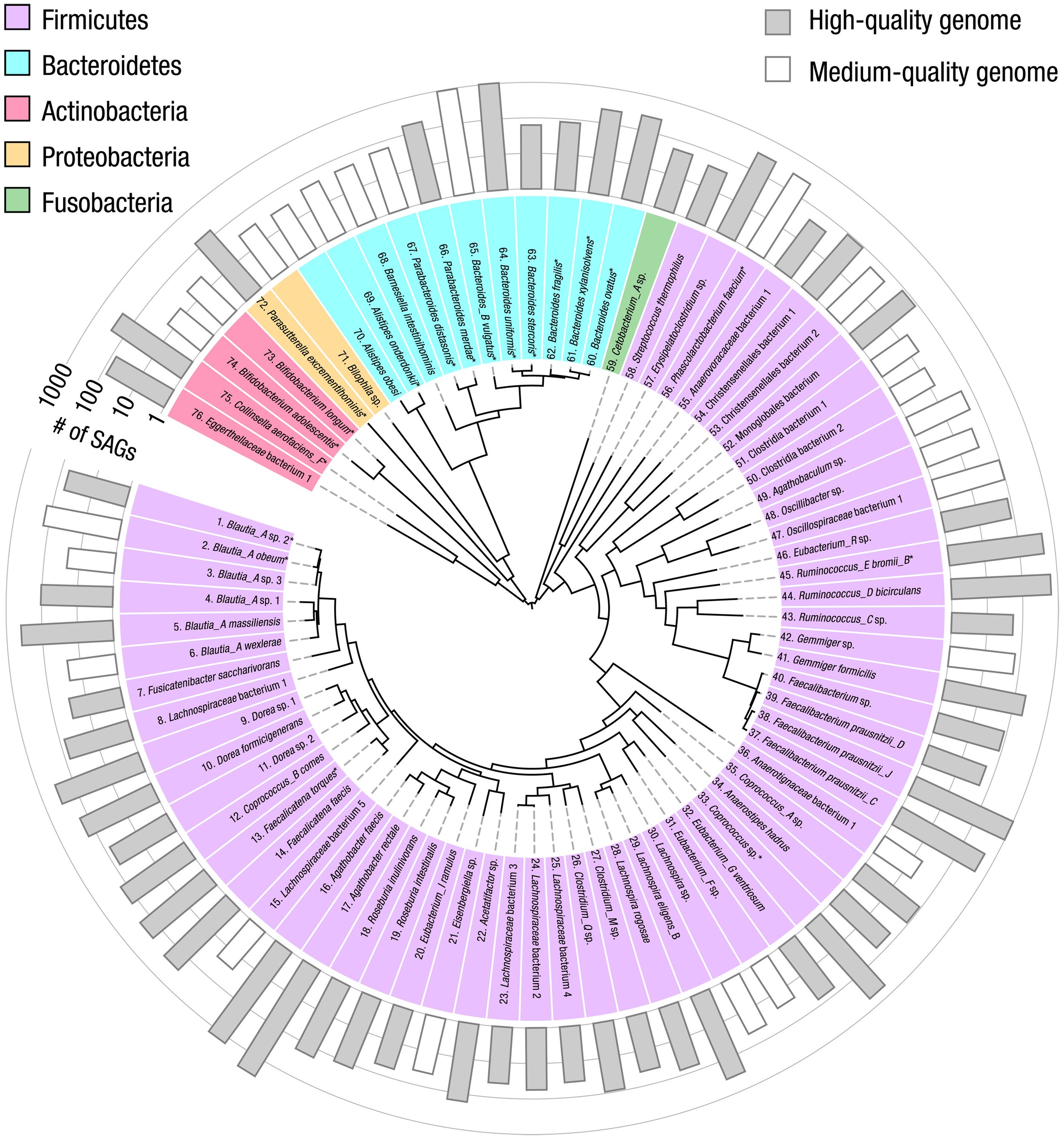
To determine whether each genome corresponds to a single species known to occur in the human gut microbiome, we compare each coassembled genome against a public database (GTDB-Tk) (59), using the ANI >95% criterion to identify matches of the same species. We obtain a broad mix of species from diverse phyla including Firmicutes, Bacteroidetes, Actinobacteria, Proteobacteria, and Fusobacteria (reported with assembly quality information in table S3). Several species well known in the human gut microbiome are abundant, including Faecalibacterium prausnitzii, Bacteroides uniformis, and B. vulgatus. For each of these 76 genomes, we list the name (colored according to corresponding phylum), illustrate its phylogenetic relationships with other species with a dendrogram, and indicate the number of SAGs used in its coassembly with the length of the outer bars, shaded for those of high quality, in Fig. 2.
Fig. 2. Coassembled genomes of 76 bacterial species in the human gut microbiome of a single human donor.
These 76 bacterial species have high- or medium-quality coassembled genomes. A phylogeny constructed from ribosomal protein sequences is represented by the dendrogram in the center of the circle. The phylum of each species is indicated by the background color behind each listed species name (GTDB-Tk database); the 19 species with genomes from isolates cultured from the same human donor are marked with an asterisk. The number of SAGs used for coassembly (abundance) is indicated by the bars in the outermost ring, shaded in gray for the 52 high-quality genomes and unshaded for the 24 medium-quality genomes.
Because there exists for these samples a large number of isolates cultured from the same human donor (12), we compare the coassembled genomes with the “gold standard” genomes derived from isolates. We find 19 species for which the coassembled genomes have corresponding isolate genomes, which we mark with an asterisk following each species name in Fig. 2. The ANI exceeds 99.5% in 17 species; these data provide strong evidence for the faithful reconstruction of genomes that closely match those of the cultured isolates, with low contamination.
With only a small set of culture-free experiments, we recover a broad set of accurate reference genomes from more species than those recovered from any other single gut microbiome. These genomes enable us to assign a large majority of single-microbe SAGs in the sample to one of these 76 species.
Microbial diversity in the human gut microbiome
Although species-level genomes provide one approach to assess microbiome diversity, the diversity of the human gut microbiome is typically assessed with metagenomics. We follow the spirit of this metagenomic approach and repurpose the droplet-based dataset to mimic that produced in metagenomics, by considering all reads from all SAGs in each sample. We classify each read in each sample by comparing it with the public database of microbial genomes (60); we also perform this comparison on each read from the corresponding metagenomic datasets (12). Each stool sample contains thousands of cells, in contrast to metagenomics which typically accumulates genomic data from millions of cells. Nevertheless, we recover 96.9 to 99.8% of the genera found by metagenomic analysis of the seven stool samples (figs. S3 and S4 and table S2).
The large collection of coassembled species-level genomes, however, provide an additional way to assess diversity with even greater precision at the species level. We align all metagenomic reads to the combined genome of all coassembled species irrespective of quality and find that 96 to 98% of these reads align, thereby providing further evidence that the droplet-based method does not miss any noticeable number of abundant taxa. For the 76 species with high- or medium-quality genome coassemblies, we estimate the relative abundance of each species in both metagenomics and the droplet-based approach. In metagenomics, the number of cells from a given species is proportional to the average read coverage over its genome; by contrast, in the droplet-based method we infer relative cell number by counting SAGs corresponding to the given species. We find that both abundance estimates are well correlated for the 76 species (fig. S5), though with one notable trend: In general, Gram-negative species—particularly those from Bacteroidetes and Proteobacteria—are underrepresented in the droplet-based method; by contrast, Gram-positive species, including Firmicutes and Actinobacteria, are overrepresented—albeit with a few exceptions (fig. S6). These trends may result from differences in lysis methods: for the metagenomics samples, we follow standard lysing protocols that use mechanical bead beating; because such mechanical methods have not been demonstrated in droplets, we use purely enzymatic methods known to favor Gram-positive species.
Strain-resolved genomes in the human gut microbiome
Many species in the human gut microbiome are represented by multiple strains (61); different strains may play distinct roles within complex microbial communities and express different sets of genes to carry out these roles (62). Linking specific genes and consequently their functionality to the strains which contain them requires knowledge of the genomes from those individual strains. Moreover, because each microbe inherently represents only a single strain, definitive identification of each SAG requires strain-resolved reference genomes.
To explore the possibility that the coassembled genomes contain contributions from more than a single strain, we further examine the comparison between the 19 coassembled genomes and cultured isolates of the same species; each of these isolates represents only a single strain. In general, the coassembled genome of a species with multiple strains contains some contigs specific to each strain; not all of these contigs appear in the single-strain genomes of the corresponding isolates. Consequently, we determine the shared genome fraction—the percentage of bases in each coassembled genome that are shared with isolate genomes from the same species. We find that for the comparison in 16 species, the shared genome fraction is above 96% and the ANI value exceeds 99.9%; these data suggest that each of these 16 coassembled genomes represents a single strain. By contrast, for the remaining three species, Blautia obeum, B. vulgatus , and Parasutterella excrementihominis, the shared genome fraction is far lower (between 70 and 90%) and ANI are all <99.6% (fig. S7). These lower values suggest that the genomes of these three species may include multiple strains or strains that do not appear among the cultured isolates. In principle, directly comparing all pairs of SAGs to estimate the fraction of their shared genomes could distinguish strains. However, the coverage of each SAG is expected to be <25% on average, for example 7% of the genome for B. vulgatus. This coverage suggests that such pairwise comparisons will not be reliable and instead motivates a different approach.
To distinguish strains, we develop a method that leverages the differences among homologous sequences between SAGs, specifically the single-nucleotide polymorphisms (SNPs). To illustrate this method we examine ~900 SAGs of B. vulgatus—the most abundant of the three species—and align reads from each SAG against the coassembled B. vulgatus genome, then identify ~12000 total SNP locations. For each SAG, we determine the SNP coverage, the fraction of all SNP locations in the genome that occur among the reads of that SAG; this SNP coverage is 8% on average, comparable to the average genome coverage. For each pair of SAGs, we measure the fraction of total SNP locations that occur in both and find this fraction to be ~0.7%, corresponding to ~80 SNPs, which is consistent with roughly the square of the SNP coverage. Microbes of the same strain have nearly identical genomes (12, 14) such that two SAGs representing the same strain almost always have the same base at each SNP location shared by both SAGs; conversely, SAGs representing different strains show considerably lower similarity (61). Inferring the similarity of the bases at shared SNP locations in each pair of SAGs is governed by a binomial process; therefore, the average of 80 SNPs in each SAG pair should be sufficient for a robust inference, with an uncertainty of 6% or less. Consequently, the comparison of SNPs provides a promising approach to determine strains.
To test this possibility, in all pairs of SAGs, we examine the bases at all shared SNP locations and determine the fraction of locations where both SAGs have the same base. To probe whether these SAGs fall into any distinct groups, we visualize the SNP similarity between all pairs of SAGs with dimensional reduction (63). Notably, we find that the SAGs fall into four clearly distinct clusters as shown in Fig. 3A. We independently validate the presence of these SAG groups with hierarchical clustering, which yields the same groupings with 99.8% overlap (fig. S8).
To test whether these clusters correlate with different strains, we examine the bases at SNP locations within each SAG cluster. We determine which base occurs most frequently at each SNP location; the set of these bases at each SNP location forms the consensus genotype of each SAG cluster. Then, for each SAG, we calculate the fraction of its SNPs that have the same base at the corresponding location in the consensus genotype of each of the four SAG clusters. Within each SAG cluster, we find that constituent SAGs share extremely high SNP similarity with the corresponding consensus genotype. For example, in the two clusters with the highest number of SAGs, almost all have the same base in >99% of the SNP locations as shown in the scatterplot and histograms in Fig. 3B. By contrast, SAG clusters show much lower overlap with the consensus genotypes of other clusters; for the two clusters with the highest number of SAGs, all SAGs in each cluster share fewer than 10% of the bases at SNP locations with the consensus genotype of the other cluster, as shown in the figure. These trends persist among the other clusters (fig. S8). Together, these results provide strong evidence that SAGs within these clusters represent the same strain.
To further examine whether these four clusters correspond to actual B. vulgatus strains, we coassemble the reads within each SAG cluster. We obtain high-quality genomes for the two groups with the most SAGs, which we label candidate strains A and B; one medium-quality genome, C; and one additional genome of lower quality, D (table S4). We compare these coassembled genomes with the genomes of two distinct B. vulgatus isolate strains cultured from the same human donor (12). We find that both isolate genomes have closely matching coassembled counterparts (A and C) with ANI values and shared genome fractions exceeding 99.9 and 97%, respectively, as shown in Fig. 3C. These high values are consistent with those that occur between genomes of the same strain, thereby providing strong evidence that these coassembled genomes each represent a single, genuine strain of B. vulgatus. Notably, the second-most populous cluster—candidate strain B, with several hundred SAGs—does not appear among the nearly one hundred isolates of B. vulgatus cultured from the same human donor (12). Together these results demonstrate the capabilities of this SNP-based approach to correctly identify both the major known strains of B. vulgatus and potential new strains that have not been cultured, while at the same time enabling the accurate coassembly of their genomes.

Fig. 3. Strain-resolved genomes of B. vulgatus in the human gut microbiome.
(A) Dimension-reduction (UMAP) visualization of B. vulgatus SAGs, based on comparison of their sequences at SNP locations. SAGs fall into four distinct, widely separated clusters; the symbol for each SAG is colored according to the cluster in which it is grouped. (B) Scatterplot and histograms illustrating the fraction of SNPs from each SAG that match consensus genotypes for SAGs in the two most abundant clusters, A and B. In almost all cases, each SAG shares the same base in more than 99% of the SNP locations in its corresponding consensus genotype; by contrast, the SNP overlap with the consensus genotype of the other cluster is much lower, typically 5% or less. The symbols in each cluster are colored as in (A). (C) Phylogeny of the coassembled high- and medium-quality genomes of B. vulgatus strains and comparison with the corresponding genomes of strains of isolates cultured from the same human donor. The horizontal axis of the dendrogram represents the ANI values between these strain-resolved genomes, demonstrating that coassembled strain C and isolate S1 are the same strain; similarly, coassembled strain A and isolate S2 are the same strain. By contrast, the second most-abundant strain, B, does not appear among the isolates cultured from the same human donor. (D) Relative abundance of the four B. vulgatus strains in the seven longitudinal samples.
We further apply this SNP-based analysis to the remaining species with high- or medium-quality species-level genomes. We find nine additional species with multiple strains and coassemble their genomes (fig. S9 and table S4). We compare the genotype of each SAG to its corresponding strain-resolved consensus genotype and observe that <1% of the SAGs have <95% similarity with the consensus genotype (fig. S10); these results are similar to those from B. vulgatus and provide strong confirmation that the separation of SAGs from different strains are robust. In total, we obtain 86 high- and medium-quality strain-resolved genomes from 76 species—from just one set of experiments—and compare to corresponding isolate genomes cultured from the same human donor. We find excellent agreement for B. obeum, with an ANI of 99.9% and shared genome fraction of 95%; this again confirms—just as in the case for B. vulgatus—that the coassembled genome represents a single, genuine strain (for the remaining multistrain species, we have no isolate genomes of the same strains with which to compare). Notably, we are able to achieve this accurate identification of strains and the coassembly of their genomes even with a level of coverage that yields an average of <100 shared SNP locations between all pairs of SAGs.
The capability to identify the strain of each individual SAG also enables us to follow the relative abundances of these strains over time in the human donor, giving insight on bacterial population dynamics. The abundances of these strains appear to shift only gradually throughout the year and a half over which samples were collected; for instance, we observe quite similar abundances in B. vulgatus in the two samples collected on successive days around day 400, as shown in Fig. 3D. These observations are consistent with previous studies showing that different Bacteroidetes species can colonize the human gut for decades stably, and that different strains of the same Bacteroidetes species can coexist with stable relative abundance (64).
The results demonstrate the capability of this approach to resolve subspecies strains and reconstruct their strain-resolved genomes, even when the SAGs have coverage of only ~10% of the genome. Furthermore, the droplet-based approach can obtain strain-resolved genomes from strains which have not been cultured; this is of particular importance in the human gut microbiome, where many strains are difficult to culture. Consequently, this method contributes a new way to examine the strain-resolved structure and dynamics of the genomic information within the human gut microbiome independent of the bias imposed by what has been cultured. These high-quality, strained-resolved genomes from a broad range of strains from the gut microbiome of a single human donor not only allow greater precision in the identification of a large majority of SAGs, but further enable the probing of broader genomic aspects of the microbial community, particularly those involving microbes of different strains.
HGT within the human gut microbiome
One particularly notable genomic aspect of microbial communities is how microbes exchange genetic information; one of the most well-known mechanisms is HGT, which is frequently observed within the human gut microbiome (20, 21, 65, 66). In general, the genomes of different bacterial species will differ considerably; however, one of the major indicators of HGT is a nearly identical sequence shared between genomes from different species (21, 67). The large number of strain-resolved genomes originating from the gut microbiome of a single human donor offers the potential to detect HGT by identifying the common sequences shared between specific microbial taxa.
To explore this sequence matching approach, we designate an HGT event between genomes from two species as the presence of a common sequence of at least 5 kb with 99.98% similarity. We apply these criteria to all 57 high-quality strain-resolved genomes, filter out potential contamination due to SAG merging (fig. S11), and observe 265 HGT sequences between 90 pairs of strains from different species, which are all HGT events within the same phylum: 65 strain pairs are within Firmicutes and 25 are within Bacteroidetes.
To evaluate whether these events might be false positives caused by contamination, we align the reads from all SAGs of each species pair against each HGT sequence, and determine the fraction of all SAGs that have adequate coverage; under a null hypothesis that if an observed HGT event were in fact a result of contamination and the sequence was absent from one of the species, then only a small fraction of its corresponding SAGs would align to the HGT sequence with sufficient coverage. Instead, we find that all of the observed HGT sequences align to a number of SAGs considerably greater than that expected under the null hypothesis in both species of each pair, thereby confirming that there are no false positives (fig. S12). Furthermore, we examine the HGT sequences from the pairs of species with corresponding cultured isolates and find that 100% of the HGT sequences determined from the coassembled genomes occur in the isolate genomes of both species.
The HGT sequences we observe encode genes involved in a variety of metabolic, cellular, and informational functions (table S5); genes indicative of phage, plasmid, and other forms of mobile genetic elements exist in ~80% of the observed HGT sequences. Among the 49 species with a single high-quality strain, we observe 66 HGT events, as shown in Fig. 4A. Notably, among the species with multiple high-quality strains we observe that individual strains of Agathobacter faecis, Faecalicatena faecis, and Anaerostipes hadrus exchange genes with different Firmicutes species whereas both strains of B. vulgatus exchange genes only with the same six other Bacteroides species, as shown in Fig. 4B. Together, these data demonstrate the ability to resolve HGT to the level of individual strains.
To determine whether any of these HGT events involve more than two strains, we identify all of the genes that occur within HGT regions and count the number of strains whose HGT sequences contain each gene. We observe that approximately half of the genes are shared among three or more species, providing strong evidence that these HGT events emerged within this single human donor. Within Bacteroidetes, genes detected from HGT sequences are shared by an average of 3.2 strain-resolved genomes versus 2.6 strains within Firmicutes, as shown in Fig. 4C (table S6).
Notably, we find several genes that occur in the HGT sequences of six or seven Bacteroidetes strains. We examine the HGT sequences containing these particular genes and find that these sequences are connected with an integrative conjugative element containing a type VI secretion system (T6SS), consistent with previous analysis using cultured isolates of Bacteroides from the same human donor (14); T6SS is one of the most-studied systems in Bacteroides that mediates interstrain competition between Bacteroides strains and has been shown to transfer between members of the same microbiome. In Firmicutes, we also observe genes shared among HGT sequences of six different strains; these HGT sequences contain genes annotated as recombinase, suggestive of an integrative mobile element or prophage.
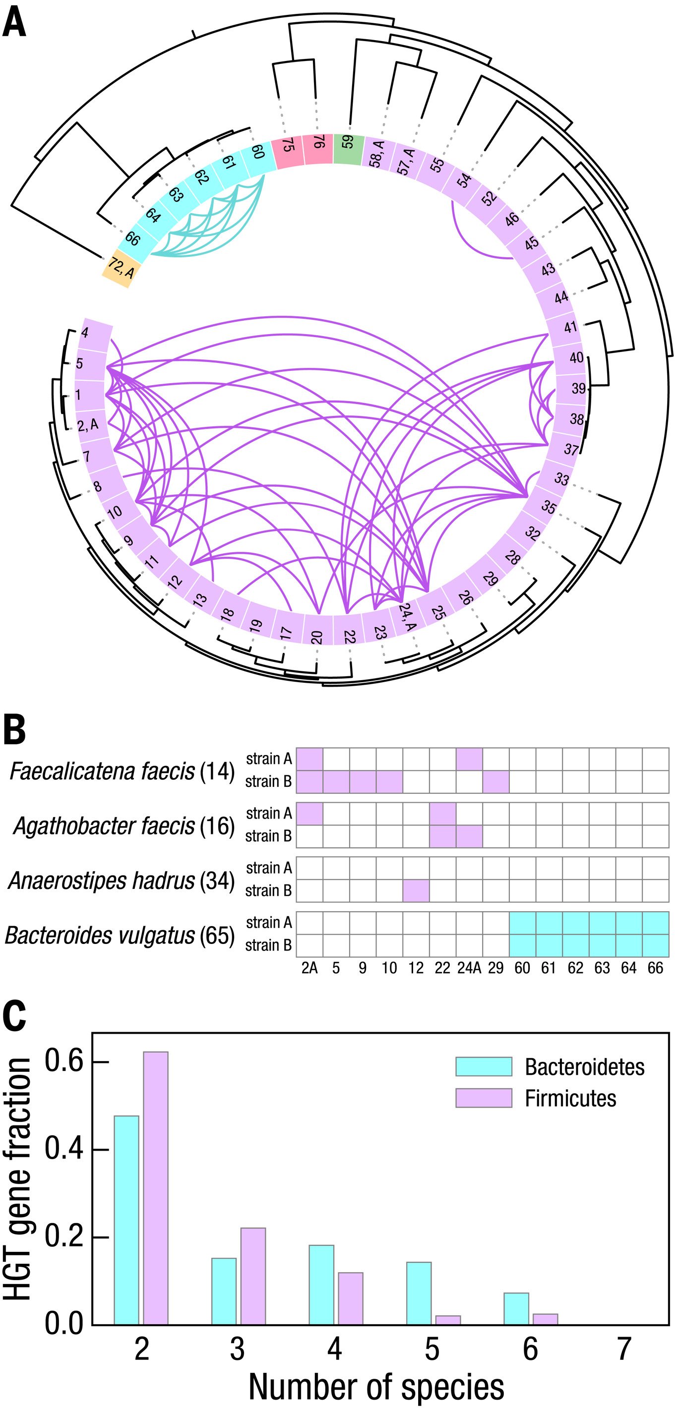
Fig. 4. HGT among bacterial strains within the human gut microbiome of a single donor.
(A) HGT among the 49 species with a single high-quality strain-resolved genome, following the order, numbers, and colors of Fig. 2. Detected HGT between two genomes indicated with a curve whose color matches that of the phylum of each species pair. (B) HGT between species with multiple high-quality strain-resolved genomes and species with single high-quality strain-resolved genomes, following the numbering in (A). For the bacteria in phylum Firmicutes (Agathobacter faecis, Faecalicatena faecis, and Anaerostipes hadrus), each strain has HGT with different sets of species. For the phylum Bacteroidetes, the only multistrain species is B. vulgatus, which has HGT between both of its strains and all other species in this phylum. (C) Distribution of the number of species in which HGT genes are shared. Approximately half of the genes in these HGT sequences are shared among more than two species; several genes occur in six or seven bacterial strains.
Together, these data provide strong evidence that our methodology detects HGT widely and robustly, among strains of many species from multiple phyla within the gut microbiome of a single human donor. The detection of HGT among six or more species within this single microbiome suggests that HGT may have important functional consequences to the recipient strains. These methods provide new tools to investigate the interactions of multiple microbes within the human gut microbiome.
Host-phage association in the human gut microbiome
The ability to investigate microbial interactions within the human gut microbiome is not limited to only bacteria, but also includes other types of microbes. Indeed, the diversity analysis reveals the presence of viruses—specifically crAssphage, the most abundant bacteriophage recognized at present from the human gut microbiome (68, 69). The general regulatory role of bacteriophages, thought to modulate the abundance and behavior of bacteria, is only beginning to be understood within complex microbial communities (70, 71). The droplet-based method encapsulates not only an individual bacterium but also any bacteriophages physically colocated with it, providing a direct means to probe host-phage association. To explore this association, we compare the reads in each SAG to the crAssphage genome; we find that a few dozen SAGs contain a substantial fraction of crAssphage-aligned reads. Moreover, many of these SAGs also contain a significant fraction of reads which do not align to the crAssphage genome but instead to bacterial taxa; we align these reads against the coassembled genomes of 76 species to identify which, if any, bacterial species might associate with crAssphage strain in this particular human donor.
Significantly, we find that 14 SAGs are associated with only one species, B. vulgatus (P value = 4 × 10⁻⁹, Fisher’s exact test) (table S7) and that no other species associates significantly with crAssphage, as shown in Fig. 5A. These data strongly suggest B. vulgatus as the in vivo host species for crAssphage in this human donor, consistent with previous evidence that crAssphage is likely to be associated with Bacteroides species (68, 72). The statistical significance of the association indicates that this is not a result of simple random coencapsulation.
Furthermore, the unambiguous assignment of each SAG to one of the multiple strains of B. vulgatus enables even more precise characterization of in vivo host-phage association to the level of specific bacterial strains. We find that 13 SAGs represent the single B. vulgatus strain A, the most abundant (P value = 3 × 10⁻¹¹), as shown in Fig. 5B.
These data demonstrate the unique advantages of the droplet-based approach to establish accurate in vivo host-phage association not only for an individual species but even more precisely to a specific strain. We identify which bacterial strains interact with bacteriophages and which strains do not; the genomic differences between these strains provide preliminary data that may contribute to understanding of the molecular mechanisms underlying these host-phage interactions and their longitudinal dynamics in the human gut microbiome.

Fig. 5. Host-phage association with strain specificity in the human gut microbiome.
(A) Association between the bacteriophage crAssphage and bacterial species with high- or medium-quality genomes, with species numbers as in Fig. 2. All P values are calculated with one-sided Fisher’s exact test. The only bacterial species that is significantly associated with crAssphage is B. vulgatus. (B) Association between the four strains of B. vulgatus and crAssphage. Only one specific strain of B. vulgatus—the most abundant strain, A—is significantly associated with crAssphage.
Discussion
Using Microbe-seq, a high-throughput method combining experiment and computation for single-microbe genomics, we obtain—without culturing—the genomic information of tens of thousands of individual microbes and de novo coassemble the strain-resolved genomes from 76 species, a large fraction of which have not been cultured. This high-throughput microfluidics-based approach allows for more practical individual examination of a sufficient number of microbes to achieve these results, even with an average coverage of less than a quarter of the genome. The close agreement with strains for which we have corresponding cultured isolates confirms the accuracy of this approach. These strain-resolved genomes enable the reconstruction of an HGT network within a single human; when sampled over time, these data may allow the monitoring of microbe response, at the level of specific genes in specific strains, to selective pressures unique to that person, such as disease, diet, or antibiotic treatment. In addition, the in vivo association between specific strains of bacteriophages and bacteria could provide specific starting points to investigate how phages modulate microbial composition and possibly guide subsequent development of phage-based therapeutics.
Scaling up the analysis to examine an order of magnitude (or more) microbes from complex microbial communities would shed light on important questions without requiring any other qualitative changes to the existing procedures. In the human gut microbiome, sequencing hundreds of thousands of cells would likely allow for identification of nearly all of the present species and strains, thereby enabling far more accurate surveys of diversity and abundance. Moreover, expanding the present investigation to a larger population of humans could allow direct exploration of the effects on human health of key microbial pathways and genes, opening up potential directions for future therapeutic developments.
We envision several routes for further technical improvement. Integrating long-read sequencing technologies are likely to lengthen the coassembled contigs considerably, improving the quality and completeness of resulting genome assemblies (28). Exploring additional lysis conditions would improve the evenness and efficiency of lysis, potentially allowing investigation of microbes in other phyla or even other kingdoms such as fungi. Combining these methods with functional sorting, such as IgA bind-and-sort, would correlate functional outcomes with strain-level genomic information and single-cell resolution.
Microbe-seq provides a particularly effective and practical approach in a single laboratory-scale experiment to identify and sequence fully all of the major strains in microbial communities beyond the human gut microbiome, without any a priori knowledge of constituent microbes. The practical improvements provided by our methodology may make feasible the investigation of microbial communities that affect the environments, lives and health of human communities that otherwise lack access to the resources to even begin to investigate these effects.
Materials and methods
Experimental model and subject details
We obtain stool samples from OpenBiome, a nonprofit stool bank, under a protocol approved by the institutional review boards at MIT and the Broad Institute (IRB protocol ID # 1603506899). The subject is a healthy male, 28 years old at initial sampling, screened by OpenBiome to minimize the potential of carrying pathogens and de-identified before receipt of samples. We homogenize stool samples from this donor, mix with 25% glycerol, and freeze at −80°C. For each experiment, we wash 1-3 μL of stool sample in 1 mL 1X PBS three to five times and resuspend it in 1X PBS with 15% (v/v) Optiprep density gradient medium (Sigma-Aldrich D1556) as the microbial suspension.
Mock community
We culture four bacteria strains, Bacillus subtilis ATCC 6051-U, Escherichia coli ATCC 25922, Klebsiella pneumoniae ATCC 35657, and Staphylococcus aureus ATCC 6538 in 1 mL LB liquid medium (L3522 Sigma Aldrich) overnight. We wash each bacterial culture with 1 mL 1X PBS three to five times and resuspend bacteria in 1X PBS with 15% (v/v) Optiprep density gradient medium (Sigma-Aldrich D1556). We combine approximately the same volume of these four bacterial strains and dilute to a final concentration of 5-50 million microbes/mL.
Microfluidic device fabrication
We print the device designs (fig. S1) as photomasks (CAD/Art Services, Inc.), and fabricate devices according to well-established soft-lithography procedures (73). We use photolithography and the photomasks to transfer each device design to a silicon wafer with SU8 photoresist. We cast polydimethylsiloxane (PDMS) (Sylgard 184) on the SU8 structure, where the SU8 structure on silicon wafer serves as a master for replica molding. We bake at 65°C for at least 2 hours to cure the PDMS and delaminate the resulting PDMS replicas off the master. We seal with glass slides (Corning, 2947) to create the microfluidic devices and make their surfaces hydrophobic by flowing Aquapel (PGW Auto Glass, LLC) through the channels. We remove excess residual Aquapel by flowing compressed air in the channels of microfluidic devices and bake the devices at 65°C overnight.
Isolation and lysis
We isolate microbes by encapsulating them into droplets with lysis reagents using a microfluidic device (fig. S1A and movie S1). We put the microbial suspension in a 1 mL syringe (BD Luer-Lok 1-mL syringe, 309628) and connect the syringe to the microbial suspension device inlet via a needle (BD Precisionglide syringe needles, Z192384-100EA, Sigma Aldrich) and polyethylene tubing (BB31695-PE/2, Scientific Commodities, Inc.). We connect similarly the lysis reagents and oil, 2% (w/v) surfactant (RAN biotechnologies, 008-FluoroSurfactant) in HFE 7500 (3M), to the device. We use flow rates of 30 μL/h for the microbial suspension, 120 μL/h for lysis reagents, and 300 μL/h for the oil. We collect droplets from the device outlet into a PCR tube and replace the oil from the bottom with 100 μL of 5% (w/v) oil. We add 100 μL mineral oil (MI499, Spectrum Chemical MFG Corp.) on top of the emulsion to avoid the evaporation of the aqueous phase in the droplets. We remove most of the oil from the bottom of the tube and incubate to lyse the microbes inside droplets.
We prepare an 80 μL lysis reagent mix for each experiment: 10 μL green buffer (prepGEM Bacteria, PBA 0100), 1 μL lysozyme (prepGEM Bacteria, PBA 0100), 1 μL prepgem (prepGEM Bacteria, PBA 0100), 1 μL lysostaphin (1 mg/ml in 20 mM sodium acetate, pH 4.5, Sigma, L7386), 2 μL 20 mg/mL bovine serum albumin (BSA, B14, Thermofisher), 2 μL 10% tween-20 (diluted from Tween-20, Sigma-Aldrich, P9416-50mL), 1 μL 100 uM random hexamer with the last two 3′ end bases phosphorothioated (IDT), and 62 μL water.
The incubation program for lysis is: 37°C for 30 min, 75°C for 15 min, 95°C for 5 min and sample storage at 4°C.
Whole-genome amplification
We transfer the droplet emulsion to a syringe and reinject droplets into a microfluidic merger device (48) (fig. S1B and movies S2 and S3). In the same device, we use a separate droplet maker to form droplets that encapsulate multiple displacement amplification (MDA) reagents. We synchronize the frequency of sample droplet re-injection and reagent droplet-making to form droplet pairs. Applying electric fields of 50-200 V at a frequency of 25 KHz through a pair of electrodes, we merge each droplet pair to add MDA reagents. We use flow rates of 60 μL/h for sample droplets, 100 μL/h for 2% (w/v) oil (fig. S1B, label 2), 75 μL/h for MDA reagents, and 250 μL/h for 2% (w/v) oil (fig. S1B, label 4). We incubate to amplify microbial genomes.
We prepare a 100 μL MDA mix for each experiment: 16 μL 10X phi29 DNA Polymerase Buffer (Lucigen, 30221-1), 0.5-2 μL 100 uM random hexamer with last two 3′ end bases phosphorothioated (IDT), 0.8-3.2 μL 25 mM dNTPs (Thermo Fisher, R1121), 8 μL phi29 DNA Polymerase (Lucigen, 30221-1), 2 μL 20 mg/mL bovine serum albumin (BSA, B14, Thermofisher), and we add water to make the total volume to 100 μL.
The incubation program for MDA is: 30°C for 6-8 hours, 65°C for 10 min and sample storage at 4°C.
Tagmentation
We merge sample droplets with droplets containing commercially available tagmentation reagents (Nextera), utilizing a different droplet merger device (fig. S1C and movies S4 and S5). We use flow rates of 25 μL/h for sample droplets, 100 μL/h for 2% (w/v) oil (fig. S1C, label 2), 75 μL/h for tagmentation reagents, and 300 μL/h for 2% (w/v) oil (fig. S1C, label 4). We incubate to tagment these DNA products.
We prepare a 90 μL Nextera mix for each experiment: 60 μL TD Tagment DNA Buffer (Illumina, 15027866), 12 μL TDE1 Tagment DNA Enzyme (Illumina, 15027865), 1.8 μL 20 mg/mL bovine serum albumin (BSA, B14, Thermofisher), 1.8 μL 10% tween-20 (diluted in water from Tween-20, Sigma-Aldrich, P9416-50mL), and 14.4 μL water.
The incubation program for tagmentation is: 55°C for 10 min, and sample storage at 10°C.
Bead synthesis
We synthesize beads used for combinatorial barcoding by adopting a previously reported method (44, 74). In brief, we make droplets containing acrydite-modified DNA oligos using a photo-cleavable linker (table S8, Hydrogel DNA primer, IDT) and acrylamide:bisacrylamide solution. We keep these droplets at 65°C overnight to polymerize them into uniform soft gel beads covalently bonded to the DNA oligos by photo-cleavable linkers. We extend DNA oligos on beads enzymatically with a two-step split-and-pool synthesis protocol to prepare beads with a diverse barcode sequence library. At the first split-and-pool synthesis step, we evenly split beads into a 96-well plate where each well contains a unique barcode-1 oligo (table S8, IDT). We anneal these oligos with hydrogel oligos and extend them with Bst 2.0 DNA polymerase (M0537L, NEB). After the first split-and-pool synthesis step, we pool beads, wash them and evenly split them into a 384-well plate where each well contains a unique barcode-2 oligo (table S8, IDT). We perform the second barcode strand synthesis in the same way as we extend the first barcode strand. We avoid exposing beads to strong light.
Each soft gel bead has millions of primers with the same sequence. Each full sequence contains two barcode regions: the first region has a diversity of 96; the second region, 384. Overall, the barcoding bead library has 36864 (96×384) possible sequences.
Bead preparation for barcoding
We wash 200 μL of beads with 1 mL bead wash buffer (10 mM pH 8.0 Tris-HCl, 0.1 mM EDTA and 0.1% (v/v) Tween-20), three times in a tube. We withdraw supernatant from the top, leaving 500 μL in the tube. We add 300 μL water and 200 μL 5X Phusion HF detergent-free buffer (F520L, Thermo Fisher) to the tube. We vortex the beads and keep them at room temperature for 1 min. We centrifuge beads, remove supernatants, and use these beads for barcoding.
Barcoding
We merge sample droplets with droplets containing PCR reagents and a barcoding bead, using a droplet-merger microfluidic device (fig. S1D and movies S6 to S8). We use flow rates of 50 μL/h for sample droplets, 100 μL/h for 2% (w/v) oil (fig. S1D, label 2), 15-25 μL/h for beads, 140 μL/h for PCR reagents, and 400 μL/h for 2% (w/v) oil (fig. S1D, label 5). We release barcode oligos from beads by exposing droplets to UV light (365 nm at ~10 mW/cm2, BlackRay Xenon Lamp) for 10 min. We perform PCR to barcode the DNA in the droplets.
We prepare a 240 μL PCR mix for each experiment: 136 μL water, 68 μL 5X Phusion HF detergent-free Buffer (F520L, Thermo Fisher), 8 μl 10 mM dNTPs (diluted from 25 mM dNTP mix, Thermo Fisher, R1121), 16 μl 10 μM RNS primer (table S8, IDT), 4 μl Phusion high-fidelity DNA polymerase (F530L, Thermo Fisher), 4 μl 20 mg/mL bovine serum albumin (BSA, B14, Thermofisher), 4 μl 10% tween-20 (diluted from Tween-20, Sigma-Aldrich, P9416-50mL).
The incubation program for barcoding is: 72°C for 4 min, 98°C for 30 s; 10 cycles of 98°C for 7 s, 60°C for 30 s and 72°C for 40 s; 72°C for 5 min, and sample storage at 4°C. We use slow ramping of 2°C/s at this step.
We observe the merger of some droplets after PCR, possibly during the high-temperature stage of PCR; such larger droplets may contain DNA from multiple microbes. We remove most of these droplets with droplet-size filter microfluidic device (75) (fig. S1E, movies S9 and S10) with flow rates of 120 μL/h for sample droplets and 2 mL/h for 2% (w/v) oil.
Droplet pooling and sequencing library preparation
We break the emulsion of droplets by adding 200 μL 20% (v/v) PFO (1H,1H,2H,2H-Perfluoro-1-octanol, 370533 Sigma Aldrich) in HFE 7500 (3M) into each sample after PCR. We purify the aqueous phase with 1.1X volume AMPure beads (A63881, Beckman Coulter) and resuspend into 32 μL DNA suspension buffer (10 mM pH 8.0 Tris-HCl and 0.1 mM EDTA). We use PCR to add sequencing adapters for sequencing (Illumina) and a sample index (Nextera index) to each purified DNA sample so we can sequence multiple samples in one sequencing run.
We prepare a 50 μL PCR mix for each experiment: 2.5 μL water, 10 μL 5X Phusion HF detergent-free Buffer (F520L, Thermo Fisher), 1 μl 10 mM dNTPs (diluted from 25 mM dNTP mix, Thermo Fisher, R1121), 2 μL 10 uM P5PE1 primer (table S8, IDT), 2 μL Nextera i7 primer (Illumina), 0.5 μl Phusion high-fidelity DNA polymerase (F530L, Thermo Fisher), and 32 μL DNA sample in DNA suspension buffer.
The incubation program for PCR is: 98°C for 30 s; 5-10 cycles of 98°C for 7 s, 60°C for 30 s, and 72°C for 40 s; in the end, 72°C for 5 min and sample storage at 4°C.
We purify samples with 0.8X volume AMPure beads (A63881, Beckman Coulter) and resuspend DNA products into 20 μL DNA suspension buffer (10 mM pH 8.0 Tris-HCl and 0.1 mM EDTA). We store these products at -20°C before sequencing.
Illumina sequencing
We sequence at depths ranging between ten thousand and two hundred thousand reads for each microbe. A custom read-1 primer (table S8, IDT) is required for the sample to be sequenced. For a 100 base-pair (bp) sequencing run, we use the following sequencing length configurations: read-1 sequence: 45 bp, which contains the barcode sequence; index-1 sequence: 8 bp; read-2 sequence: remainder, which contains the microbial sequence. For a 300 bp sequencing run, we use the following sequencing length configurations: read-1 sequence: 150 bp, the first 45 bp are barcode sequences, the last 75 bp are microbial sequences, and those in the middle are adapter sequences; index-1 sequence: 8 bp; read-2 sequence: remainder, which contains the microbial sequence.
Preprocessing of raw sequencing data
We group raw sequencing reads based on the 36864 barcodes, excluding barcodes associated with too few reads (~15% of total reads) and those with significantly more reads than other barcodes likely due to droplet merging (~5% of total reads). For the remaining barcodes, we designate the collection of microbial sequences associated with a single barcode as a single amplified genome (SAG). We use Trimmomatic (76) (version 0.36, LEADING:25 TRAILING:3 SLIDINGWINDOW:4:20 MINLEN:30) to remove low-quality reads and adapter sequences from each SAG for following analysis.
Mock sample alignment, quality assessment, and coverage
We use Bowtie2 (52) (version 2.2.6, default parameters) to align reads from each SAG to the combined genome of the four reference genomes (RefSeq: GCF_002055965.1, GCF_004151095.1, GCF_001936035.1, GCF_002025145.1), which reports the best hit of each read. We use SAMtools (77) (version 1.9) to check the number of reads that align to each of the four genomes and to calculate the purity of each SAG. For each SAG with high purity (>0.95), we align its reads to the most-aligned reference genome to determine its genome coverage.
Genome coassembly of microbial species in the human gut microbiome
We use SPAdes (53) (version 3.13.0,–sc–careful) to de novo assemble genomes from the reads of each of the 21914 SAGs. We compute and compare signatures of these assembled genomes using sourmash (78) (version 2.0, k-mer 51, default setting), which produces a matrix of estimated similarities between genomes. We use a hierarchical clustering method (SciPy version 1.1.0, method: complete, metric: Euclidean, criterion: “inconsistent”, and threshold: 0.95) to group SAGs into bins. We verify 0.95 as a threshold using mock samples. This set of parameters groups bins conservatively, minimizing the improper grouping of SAGs from different species. We use all the reads within each bin to coassemble a tentative genome, compare tentative genome similarities, and cluster the bins. We iterate this process until more than 10% of the assembled genomes have more than 10% contamination (estimated by CheckM version 1.0.13, default parameters) (56), which implies false clustering of SAGs; through four rounds, we group the 21914 SAGs into 364 bins.
To split bins that might contain SAGs from multiple species, we examine contig alignment patterns. Within each of the 364 bins, we align reads from each SAG to the de novo coassembled genome from that bin using bowtie2 (52) (default parameters). For each contig in the tentative genome with more than 1000 bp, we construct a vector for each contig with the number of reads aligned to the contigs from each SAG. We use a hierarchical clustering method (method: ward, default parameters) to group vectors of contigs into two groups. For each SAG, if >95% aligned reads are aligned to one of the two groups of contigs, it is designated as a SAG associated with that group of contigs. We assume that the remaining SAGs are a mixture of multiple species and exclude them from further analysis. We iterate this binary splitting process until we exclude more than 60% of the SAGs in the current bin, or both resulting new bins have fewer than 10 SAGs, or the change between the resulting new bin and the current bin is fewer than three SAGs. Using this process, we obtain 400 bins whose constituent SAGs we expect to represent a single species, with minimal contamination.
To combine bins of the same species for genome assembly, we use fastANI (55) (version 1.2, default parameters) to calculate average nucleotide identity (ANI) between all pairs of these 400 bins. Applying the commonly used ANI > 95% threshold, above which two genomes are considered to represent the same species, we generate 234 new species-level bins. We de novo assemble reads from all SAGs within each of these 234 bins and remove contigs shorter than 500 bp. To further eliminate contigs that may originate from other species within each genome, e.g., as a result of random contamination in individual SAGs, we fit a normal distribution with the coverage of contigs on a log scale and remove those contigs with coverages that are more than two standard deviations away from the mean of the distribution.
Among these 234 genomes, 76 genomes are of high-quality (>90% completeness and <5% contamination) or medium-quality (>50% completeness and <10% contamination), as assessed by CheckM (56) (default parameters). We use fastANI (55) (default parameters) to compare the genomes of these 76 bins to all microbial genomes (RefSeq as of September 2019), and to the published collection of more than a thousand cultured-isolate whole genomes (12). We identify the closest corresponding species-level genomes with ANI > 95% in both databases. The closest genomes in RefSeq to species Alistipes onderdonkii, Bacteroides fragilis, and Bacteroides ovatus are cultured isolate whole genomes from the same donor, reported previously (79); we exclude these three genome pairs from the ANI and shared genome fraction analysis (fig. S7). We use BLASTn (BLAST+, version 2.10.0) (80) (default parameters) to compare overlapping sequences between genome pairs.
The names of the species-level genomes in RefSeq are not always labeled consistently; for example, we have four species that are named as Blautia obeum in RefSeq, though their ANI values are less than 95%. We use both GTDB-Tk (59) (version 1.0.2, reference data version r89) and comparison to RefSeq genomes (as of September 2019) to assign taxonomies to all species. In the main text, we use taxonomies classified with GTDB-Tk and remove subgenus names, such as “A”.
Phylogeny analysis of genomes
To construct the phylogeny of the 76 species with high-quality or medium-quality genomes, we extract amino acid sequences of six ribosomal proteins (Ribosomal_L1, Ribosomal_L2, Ribosomal_L3, Ribosomal_L4, Ribosomal_L5, and Ribosomal_L6), concatenate and align them with Anvi’o (version 6.1) (81). We construct a maximum likelihood tree with RaxML (82) (version 8.2.12, standard LG model, 100 rapid bootstrapping). We use iTOL (version 5.5) (83) to visualize and annotate the resulting dendrograms.
Diversity of the human gut microbiome samples
For each of the seven samples, we temporarily ignore the barcode information and combine all reads from all SAGs from the sample. We use Kraken2 (84) (version 2.0.8, default parameters) to classify reads from each Microbe-seq dataset and corresponding metagenomic dataset (12) (standard Kraken database as of April 2019). For the analysis shown in fig. S4, we keep only the reads classified to a specific genus and use only this genus-level information for the comparison; similar analyses using all operational taxonomic units (OTUs) show similar results (table S2). For each metagenomic dataset, we align reads to the combined genome coassemblies from the 364 bins, irrespective of whether the bin is species level. Metagenomic reads are first quality filtered with fastp (version 0.12.4, parameters: -f 15 -t 15 -q 36 -u 10) and then aligned to the combined genomes using bowtie2 (parameter:–very-sensitive-local). We obtained overall alignment rates of 98.26%, 98.74%, 98.63%, 96.65%, 96.63%, 96.11%, and 98.64% for each of the seven metagenomic samples.
Abundance bias between Microbe-seq and metagenomics
We compare relative abundance from the 76 species with high- or medium-quality genome coassemblies. We estimate the cell number for each species in the metagenomic dataset by aligning metagenomic reads to each species-level reference genome and computing the average sequencing depth between the 20th and 80th percentiles in genome-wide sequencing depth. We infer cell number in the Microbe-seq dataset by counting the number of SAGs that we assign to each species; we normalize this cell-number inference across all these species and average across the seven longitudinal samples to obtain a single relative abundance inference for all species.
Differentiating strains of the same species
We use B. vulgatus as an example in the main text to illustrate the strain differentiation workflow; we use the same computational pipeline for all other species, without changing parameters, to resolve their constituent strains. The uncertainty in similarity of the bases at shared SNP locations in each pair of SAGs is the standard deviation of the normal approximation of the binomial distribution: uncertainty = sqrt[p(1−p)/n], where p is the probability of the event and n is the number of events. In the case of B. vulgatus, n=80 and the uncertainty is <6%.
Within each of the species with high- or medium-quality species-level genomes, we align (52) each SAG to the assembled genome. We use bcftools (77) (mpileup, filters: snps and %QUAL>30) to identify high-quality single-nucleotide polymorphism (SNP) mutations. We designate a SAG with fewer than 2 reads aligned to a SNP, as well as fewer than 99% of its reads being the same at a SNP as unknown/unaligned at this location. We remove SNPs with fewer than 5% of SAGs aligned to the location, and SNPs with fewer than two SAGs being the reference allele or fewer than two SAGs being the mutation allele. We also remove any SNP with fewer than 1% SAGs being the reference allele or fewer than 1% SAGs being the mutation allele. We remove any SAG that covers less than 1% or fewer than 10 of the kept SNP locations.
We identify thousands of SNP locations and remove up to 6% of SAGs. We construct a SNP vector to represent the base identity sequence of each SAG at each SNP location. To identify the number of strains of the species in the samples, we build a dendrogram of SAGs with hierarchical clustering (method: “ward”) using the SNP vectors of all SAGs. Although the number of clusters is not obvious from the dendrogram, we obtain a sequence of SAGs; in this sequence, SAGs with similar SNP sequences are closer. We compare similarities of SNP vectors between SAGs at their shared SNP locations and construct a similarity heatmap with SAGs ordered in the same sequence as the corresponding dendrogram. We observe block-diagonal squares in the heatmap, which indicates that SAGs within each square are closer to each other than to SAGs in other squares. Using the block-diagonal squares in the heatmap, we determine the number of strains, though this number is challenging to determine accurately for species with relatively few SAGS (<200) and for species with potentially more than two strains. For Blautia obeum, it is unclear whether there are 3 or 4 strains in the sample; for Parasutterella excrementihominis, it is unclear whether there are 2 or 3 strains. We apply UMAP (63) (default parameters) to the SNP data to create dimensional-reduction plots (fig. S9).
To remove SAGs that have reads from microbes of multiple strains, we construct the consensus genotype of each strain by comparing the SNP vectors of SAGs of the same strain. If more than 90% of the values at a SNP location from all SAGs within the strain are the same, we use the value for this SNP in the consensus genotype for the strain; otherwise we drop this SNP location for this strain. We compare the SNP vector of each SAG to the consensus genotype of each strain and assign strains to those SAGs that match more than 95% locations at the consensus genotype of only one strain, which excludes fewer than about 1% of the SAGs from each species. We coassemble strain-resolved genomes with reads from all SAGs in each of these assigned strains with SPAdes (53) using default parameters.
Horizontal gene transfer analysis
We detect HGT events by searching for blocks of DNA sequences shared by a pair of strain-resolved genomes that are longer than 5000 bp and more than 99.98% identical (14, 67). Assuming that species from the gut microbiome evolve with a molecular clock of 1 SNP/genome/year and that typical genome size is 5,000,000 bp, this set of criterion detects sequences that diverged within the past 1000 years and the HGT events likely emerged within the human host, based on known mutation rates (14). To filter out HGT sequences resulting from contaminated SAGs, we select all SAGs from each strain-resolved genome, and align reads from each SAG to the corresponding strain-resolved genome. We remove SAGs with an overall sequence alignment ratio below 90%, which eliminates three HGT sequences from two genome pairs, as no SAGs from one of the strain-resolved genomes have reads that cover the HGT sequences.
To further validate the remaining detected HGT sequences, we align reads from all the filtered SAGs from both HGT-associated species. We calculate the number of SAGs belonging to each strain-resolved genome with more than 500 bp coverage over the HGT sequence. We explore the statistical likelihood of the observed fraction of SAGs containing reads covering the HGT sequence. We build a null model that if we detect an artifactual HGT event between species A and B, that sequence actually only exists in the genome of species B, but appears in the SAGs of species A as a result of contamination. We assume a worse-than-real scenario that if a SAG from species A is contaminated by species B, this SAG will contain reads covering the false HGT sequence. We also assume a worse-than-real contamination rate of 20% SAGs for any strain and species. Under these assumptions, the upper limit for the probability that any SAG from species A is contaminated by B is: 20% × (relative abundance of B) = 0.2 × Nb / N, where Nb is the number of SAGs from species B, and N is the total number of SAGs. If the observed SAG number for species A is Na, and the observed number of SAGs contaminated by B is up to x, then the probability that equal or more than x of the SAGs from species A are contaminated by species B is 1-binom.cdf(x, Na, 0.2×Nb/N); this calculated quantity represents the upper limit of the P value for the observed fraction of SAGs containing reads from the HGT sequences.
To explore whether these HGT events either emerged within this human subject or before both strains colonized the host, we compare our results to the baseline detectable HGT from strains that are not from the same human host. For 39 species that we find a corresponding high-quality genome assembly from the NCBI database, we select the single genome that most closely matches the strain-resolved genome from Microbe-seq using ANI. We apply our exact HGT criteria to this collection of 39 genomes from the NCBI database, and compare with the corresponding 39 strain-resolved genomes from Microbe-seq in fig. S13.
We predict genes (open reading frames, ORFs) from the HGT sequences using prokka (85), (version 1.12, default parameters). We annotate ORFs using eggnog-mapper (86) (version 3.0, parameter: -m diamond–tax_scope auto–go_evidence nonelectronic–target_orthologs all–seed_ortholog_evalue 0.001–seed_ortholog_score 60–query-cover 20–subject-cover 0). For each HGT sequence, we assign the sequence to a certain type of mobile element if ORF annotations contain signatures of mobile elements (detailed information in table S5). To examine how many species share the same HGT sequences, we cluster all the ORFs from all HGT sequences using CD-HIT (87) (version 4.7, 100% similarity). For each gene cluster, we count the number of species whose HGT sequences contain genes within the gene cluster (Fig. 4C and table S6). We cluster genes from only the HGT regions and the HGT sequences detected via our method, which are likely incomplete fragments of the original HGT events; therefore, the number of species we report for each gene is likely an underestimation.
Host-phage association analysis
To identify SAGs that are associated with both crAssphage and a bacterial cell, we use bowtie2 (52) (default parameters) to align reads in each SAG to the crAssphage genome (Refseq: GCF_000922395.1). We designate SAGs with more than 5% reads aligned to the crAssphage genome as containing significant crAssphage reads (raising this threshold to 10% of reads yields the same result); we align the non-crAssphage reads of these SAGs to each of the 76 high- or medium-quality genomes, as well as the combined genome of these 76 genomes. We define purity of these SAGs as the maximum number of reads aligned to individual genomes divided by the number of reads aligned to the combined genome. We identify SAGs with more than 50% of reads aligned to one of these 76 genomes, and with purity of more than 95%. We designate the species of the SAG as the species of the most aligned genome. We count the number of SAGs assigned to each species and perform the “one species versus remaining species” one-sided Fisher’s exact test.
Acknowledgments
We thank members of the Weitz and Alm laboratories for helpful discussions and Y. Cai, W. Chen, Z. Cheng, N. Cui, L. Dai, R. Ding, P. Ellis, Z. Ge, J. Gong, H. Li, F. Ling, B. Liu, H. Liu, H. Pei, R. Rosenthal, J. Tang, Y. Wang, J. Xia, Y. Yao, X. Yu, Z. Zhang, Z. Zhang, and Z. Zhao for general discussions and comments on the manuscript. P.J.L. acknowledges support from the Massachusetts DTA through the SNAP and HIP programs. We thank OpenBiome for providing stool samples. We thank the MIT Center for Microbiome Informatics and Therapeutics and The Bauer Core Facility at Harvard University for providing sequencing services.
Funding: This work was supported by the following: US Department of Energy, Office of Science, Office of Biological & Environmental Research, grant DE-AC02-05CH11231 at Lawrence Berkeley National Laboratory by ENIGMA-Ecosystems and Networks Integrated with Genes and Molecular Assemblies; The National Science Foundation grant DMR-1708729; The National Science Foundation grant, through the Harvard University Materials Research Science and Engineering Center, DMR-2011754; National Institutes of Health grant P01HL120839; National Institutes of Health grant R21AI125990; National Institutes of Health grant R21AI128623; National Institutes of Health grant R01AI153156; National Aeronautics and Space Administration grant NNX13AQ48G; National Aeronautics and Space Administration grant 80NSSC19K0598.
Author contributions: W.Z., S.Z., H.Z., P.J.L., E.J.A., and D.A.W. conceived and designed the methodology; W.Z. developed and performed the experiments with assistance from S.Z.; S.Z., W.Z., Y.Y., D.M.N., and C.L.D. performed the data analysis with input from all authors; P.J.L., W.Z., and S.Z. wrote the initial manuscript; D.A.W., P.J.L., W.Z., S.Z., and E.J.A. revised the manuscript; all authors read and commented on the manuscript; E.J.A. and D.A.W. supervised the study.
Competing interests: E.J.A. is affiliated with Finch Therapeutics and Biobot Analytics. All other authors declare no other competing interests.
Data and materials availability: Combined fastq files for each stool sample, with read header containing the unique SAG ID and adaptor removed and filtered for quality, are available from NCBI Sequence Read Archive (Bioproject: PRJNA803937). Metagenomic fastq files are available from the previous publication (Biopoject: PRJNA544527). Commented scripts, intermediary data, and genome coassemblies are available at (88).
License information: Copyright © 2022 the authors, some rights reserved; exclusive licensee American Association for the Advancement of Science. No claim to original US government works. https://www.sciencemag.org/about/science-licenses-journal-article-reuse