Intermittent fasting and weight loss: Systematic review

Intermittent fasting is a “trend” spoken of often in “Mom “and “health and fitness” groups. But what is it and what does the medical establishment say about the risks and benefits of intermittent fasting? Dr. Stephanie Welton and Dr. Len Kell have published in the journal of Canadian Family Physicians a systematic review of the available literature on controlled studies on intermittent fasting. Their results may surprise you.

”Weight regain did occur after 6 months. Five studies followed participants for 6 months or longer after completing IF interventions of 8 weeks to 1 year and most studies saw body weight increase by 1% to 2% of their weight nadir.”

My conclusion: More research is needed. The vast majority of studies were far less than a year in duration. If it seems too good to be true, it probably is!

AUTHORS: Stephanie Welton, Robert Minty, Teresa O’Driscoll, Hannah Willms, Denise Poirier, Sharen Madden and Len Kelly. Canadian Family Physician February 2020, 66 (2) 117-125;

Abstract

Objective To examine the evidence for intermittent fasting (IF), an alternative to calorie-restricted diets, in treating obesity, an important health concern in Canada with few effective office-based treatment strategies.

Data Sources A MEDLINE and EMBASE search from January 1, 2000, to July 1, 2019, yielded 1200 results using the key words fasting, time restricted feeding, meal skipping, alternate day fasting, intermittent fasting, and reduced meal frequency.

Study selection Forty-one articles describing 27 trials addressed weight loss in overweight and obese patients: 18 small randomized controlled trials (level I evidence) and 9 trials comparing weight after IF to baseline weight with no control group (level II evidence). Studies were often of short duration (2 to 26 weeks) with low enrolment (10 to 244 participants); 2 were of 1-year duration. Protocols varied, with only 5 studies including patients with type 2 diabetes.

Synthesis All 27 IF trials found weight loss of 0.8% to 13.0% of baseline weight with no serious adverse events. Twelve studies comparing IF to calorie restriction found equivalent results. The 5 studies that included patients with type 2 diabetes documented improved glycemic control.

Conclusion Intermittent fasting shows promise for the treatment of obesity. To date, the studies have been small and of short duration. Longer-term research is needed to understand the sustainable role IF can play in weight loss.

In 2018, 63.1% of Canadian adults were overweight or obese.1 Obesity is a risk factor for cardiovascular disease and type 2 diabetes.2,3 As obesity rates climb, there is increasing focus on dietary interventions, the most common being calorie-restricted diets, which achieve initial but often unsustained weight loss.4 There is recent interest in the use of fasting for the treatment of obesity5–7 and diabetes.8,9 Intermittent fasting (IF) refers to regular periods with no or very limited caloric intake. It commonly consists of a daily fast for 16 hours, a 24-hour fast on alternate days, or a fast 2 days per week on non-consecutive days.8 During fasting, caloric consumption often ranges from zero to 25% of caloric needs. Consumption on nonfasting days might be ad libitum, restricted to a certain diet composition, or aimed to reach a specific caloric intake of up to 125% of regular caloric needs.9 Various terms are used to describe regular intermittent calorie abstention, including intermittent fasting, alternate-day fasting, reduced meal frequency, and time-restricted feeding. Intermittent fasting can be used with unrestricted consumption when not fasting or in conjunction with other dietary interventions. This review provides the most recent evidence on IF’s effects on weight loss and the potential role it plays in primary care treatment of obesity.

DATA SOURCES

An EMBASE and MEDLINE search of articles from January 1, 2000, to July 1, 2019, returned 1200 unique results using the key words alternate day fasting, intermittent fasting, fasting, time restricted feeding, meal skipping, and reduced meal frequency. We included English-language studies that focused on weight loss for overweight and obese participants (body mass index [BMI] of ≥ 25 kg/m2) and excluded studies of very short duration (< 2 weeks), studies of those requiring inpatient treatment, or studies focused on stroke, seizures, or other specific medical conditions. Following these exclusions 41 articles remained, describing 27 unique experiments: 18 small randomized controlled trials (level I evidence) and 9 trials comparing weight after IF to baseline weight with no control group (level II evidence) (Table 1).10–50 Levels of evidence are classified according to the Canadian Task Force on Preventive Health Care.

SYNTHESIS

Study design

Study interventions incorporated IF in a variety of ways, from a 24-hour fast several days per week (eg, the “5 and 2” protocol)11,16,17,21,27,28,35,41,42,50 to a daily 16-hour fast.10,12,25,34 The most common study design was to alternate 24-hour periods of fasting with unrestricted consumption (alternating fast and feast days).13,15,19,20,22–24,29,33,38,43,47,49 Study protocols also varied in their recommendations on caloric intake, enrolment of patients with diabetes, presence of a control group, and study duration. Some studies restricted calories while others allowed ad libitum consumption when not fasting. The rigour of fasting also varied, with several studies allowing 25% of regular caloric consumption during fasting periods. Comparator groups to IF diets followed a usual diet13,20,25,43,49 or calorie-restricted diet.11,15–17,19,22,27,28,33,41–43

While patients with diabetes were commonly excluded (Table 2),10,11,13,15,19–25,27–29,32,33,35,37,38,40–43,47,49,50 5 studies enrolled only those with type 2 diabetes (n = 174 patients) (Table 3).12,16,17,21,34 In both diabetic and non-diabetic populations, cardiovascular risk factors were reduced. When diet composition was controlled, most protocols were consistent with Health Canada and American Heart Association guidelines at the time: 55% carbohydrates, 20% fat, and 25% protein.51,52 The most common alternative was unrestricted consumption. An enrichment of protein was considered in 5 studies at the expense of carbohydrate intake.12,15,16,28,50 Two followed a Mediterranean-type diet.27,42 Fat consumption was examined in 1 study, which compared dietary fat intake of 45% versus 25%, at the expense of carbohydrate intake.37 Sixteen studies included dietary education, with participants choosing their own meals, while 11 supplied all or part of the diet.1,13,19,23,29,33,34,37,43,47,49 Others did not require a specific dietary composition outside of the fasting period.

Table 2.

Outcomes of risk factors for cardiovascular disease and type 2 diabetes in 26 individual studies of 22 intermittent fasting trials enrolling obese adults without type 2 diabetes

Table 3.

Outcomes of risk factors for cardiovascular disease and type 2 diabetes in 5 intermittent fasting studies enrolling obese adults with type 2 diabetes

Studies were of limited size and duration: 18 of 27 trials analyzed fewer than 60 participants and were 12 weeks or fewer in duration. The longest studies lasted 1 year and had 137 to 244 participants.17,28 Several studies had follow-up periods after the intervention ranging from 2 weeks to 1 year.12,15,18,19,41–43,50

Weight loss

In all 27 trials (n = 944 IF participants), IF resulted in weight loss, ranging from 0.8% to 13.0% of baseline body weight (Table 1).10–50 Weight loss occurred regardless of changes in overall caloric intake.43,53 In the 16 studies of 2 to 12 weeks’ duration that measured BMI, BMI decreased, on average, by 4.3% to a median of 33.2 kg/m2.10,12,13,19–21,23–25,29,34,35,37,47,50 Waist circumference decreased by 3 cm to 8 cm in studies longer than 4 weeks that recorded it.13,21,23,24,27,33–35,37,41,42,47

Twelve studies used calorie-restricted diets as a comparator to IF and found equivalent weight loss in both groups. 11,15–17,19,22,27,28,33,41–43 Study duration was 8 weeks to 1 year, with a combined total of 1206 participants (527 undergoing IF, 572 using calorie restriction, and 107 control participants) and demonstrated weight loss of 4.6% to 13.0%.11,15–17,19,22,27,28,33,41–43 Adherence appears similar for both weight loss strategies.15,17,27,28 The largest study comparing IF with calorie restriction was by Headland et al in 2019 of 244 obese adults who achieved a mean 4.97-kg weight loss over 52 weeks versus a mean weight loss of 6.65 kg with calorie-restricted diets (P = .24).28 All of the 11 other comparisons of IF and calorie-restriction diets also found similar results between both groups.11,15–17,19,22,27,33,41–43 In several of these studies, those in the IF group consumed the same amount of calories22,41–43 or less19,27,33 than those in the calorie-restriction group. Four studies combined fasting and calorie restriction on the non-fasting days and found comparable weight loss to other studies (3.4% to 10.6%).15,23,33,35 In a direct comparison of 88 participants over 8 weeks, IF combined with restricting calories to 30% less than their calculated energy requirements led to greater weight loss versus IF alone (P ≤ .05).33

Most of the weight loss with IF is fat loss.13,17,19,20,22,28,29,33,35,43,47,53 A 2011 study by Harvie et al calculated that 79% of weight loss was owing to loss of fat specifically (level I evidence).27 Participants regained some weight during follow-up after intervention, although average body weight remained statistically significantly lower than baseline levels.15,18,19,41–43,50 Weight regain did occur after 6 months. Five studies followed participants for 6 months or longer after completing IF interventions of 8 weeks to 1 year and most studies saw body weight increase by 1% to 2% of their weight nadir.18,19,41,43,50 Catenacci et al found a mean 2.6-kg regain over 6 months,19 and Schübel et al41 and Trepanowski et al43 each found a regain of 2% of baseline body weight. The year-long study by Carter et al of 137 participants was the exception, demonstrating a maintained weight loss.18 Zuo et al saw a BMI increase of less than 1% during a year-long follow-up period after 12 weeks of IF.50 In 6 comparisons of IF and calorie restriction, the amount of weight regained after IF and calorie restriction was similar.15,18,19,41–43 The 2016 study by Catenacci et al showed differing patterns of weight regain. In the 11 IF patients who completed follow-up, this was limited to lean body mass, while the 10 calorie-restricted patients who completed follow-up regained both fat and lean body mass.19

The practical length of a fast to effect changes in weight appears to be 16 hours. In IF studies with a daily fasting intervention, a total of 120 participants were able to maintain a minimum daily fast of about 16 hours (15.8 to 16.8 hours), with an 8-hour eating window each day.10,12,25,34 Arnason et al found that participants were able to fast for an average of 16.8 hours per day, rather than the 18- to 20-hour goal they had set.12 Combining exercise with IF improved weight loss in a 2013 study by Bhutani et al of 64 obese patients. They found weight loss doubled (6 kg) when exercise was added to IF (level I evidence).13 In 2019, Cho et al found no improvement in weight loss when exercise was added to IF (n = 31) (level I evidence).20 There were high dropout rates (≥ 25%) in several IF studies,11,13,20,25,28,43,50 which compare poorly to the 12% to 14% dropout rates of other long-term diets: Atkins, Zone, LEARN (Lifestyle, Exercise, Attitudes, Relationships, and Nutrition), and Ornish.54 In direct comparisons of IF to calorie restriction, the 2 have similar dropout rates.11,15–17,19,22,27,28,33,41–43 Across the IF studies, adherence to fasting ranged from 77% to 98% (n = 265).10,11,13,17,21,29,38 In a 2009 study, Varady et al found weight loss was directly related to percentage of adherent days per week (level II evidence).47

Intermittent fasting studies generally find that hunger levels remain stable22,31 or decrease during IF.38,45 A study of 30 participants over 12 weeks by Varady et al found reports of hunger during IF were no higher than with unrestricted consumption (level I evidence).49 Kroeger et al found that among those with the highest weight losses over 12 weeks of IF, hunger decreased and fullness increased.45 In the study by Harvie et al, 15% of participants reported hunger.27 Sundfør et al saw higher reported hunger in the IF group compared with those in the calorie restriction group.42

Ramadan is a culturally determined example of IF for many Muslims. Those who fast often do so for approximately 14 hours per day for 30 days, presenting a real-world opportunity for examining effects of fasting.55–62 Eight Ramadan studies examined weight loss in obese adults (n = 856).55–62 Weight losses ranged from 0.1 kg58 to 1.8 kg61 (level II evidence). Studies enrolling participants with diabetes saw a modest improvement in glycemic control.58,60,62 Diabetes Canada issued detailed recommendations on management of patients with diabetes during Ramadan in February 2019.63 Their expert panel recommends individualized risk stratification, glucose monitoring, and treatment with medications with low hypoglycemia risk profiles.63

Diabetes

While IF is a moderately successful strategy for weight loss, it shows promise for improving glycemic control. Five studies exclusively enrolled individuals with type 2 diabetes (Table 3).12,16,17,21,34 Kahleova et al compared a daily fast of at least 16 hours to caloric restriction (n = 54).34 Both groups experienced decreases in insulin levels but IF participants had significantly lower fasting glucose levels (−0.78 mmol/L vs −0.47 mmol/L, P < .05). Increased oral glucose insulin sensitivity, decreased C-peptide levels, and decreased glucagon levels were also statistically significantly greater in the IF group. The decrease in hemoglobin A1c level was similar between the IF and calorie-restricted groups—a 0.25% decrease over 12 weeks (level I evidence).34

In a 2016 pilot study, Carter et al implemented a fast 2 days per week with an otherwise usual diet versus caloric restriction every day in participants with diabetes (n = 51).16 Medication use was reduced and hemoglobin A1c levels decreased significantly (by 0.7%) during the 12-week study (P < .001), but the effect of IF on weight did not differ from that of caloric restriction (level I evidence).16 The 2018 trial that followed (n = 137) saw the same result over 12 months of IF or calorie restriction (level I evidence).17 The improvements in hemoglobin A1c level were lost during the 12 months after IF, although weight losses and medication reductions remained.18 In the 2017 Saskatchewan study by Arnason et al, 10 participants with type 2 diabetes fasted an average of 16.8 hours per day for 2 weeks.12 They found improved glycemic control with lower morning, postprandial, and average mean daily glucose levels (level II evidence).12 These improvements regressed once participants returned to their usual diets. Corley et al enrolled 41 individuals with diabetes in a 2018 study of twice-weekly 1-day fasts for 12 weeks; fasting glucose levels decreased by 1.1 mmol/L and hemoglobin A1c levels by 0.7% (level II evidence),21 a decline similar to that in the earlier study by Carter et al.16 Kahleova et al found a more modest decrease in blood glucose levels (−0.78 mmol/L) with a daily 16-hour fast; no adverse events were reported.34

Use of IF in patients with diabetes poses a risk of hypoglycemia. Olansky suggests adjusting medication in patients with type 2 diabetes taking insulin or insulin secretagogues (eg, sulfonylureas).64 Other hypoglycemic agents such as metformin, glucagonlike peptide 1 agonists, dipeptidyl peptidase 4 inhibitors, and α-glucosidase inhibitors are considered less likely to cause hypoglycemia (level III evidence).64 Olansky indicates that adjustments might not be required to long-acting basal insulin, but that short-acting analogues should be reduced on fasting days to reflect the timing of meals and anticipated carbohydrate intake (level III evidence).64 Premixed insulins (ie, intermediate-acting and short-acting insulin) are not recommended during IF, as they are not adaptable to changes in meal timing and calories.64 Corley et al reduced any insulin use by up to 70% on fasting days.21 Hypoglycemic events (blood glucose level ≤ 4.0 mmol/L) in that study (n = 41) were experienced on average every 43 days, with no severe hypoglycemic events (ie, requiring assistance of another person).21 Carter et al proposed lessening the risk of hypoglycemic events through pretrial discontinuation of all insulin and sulfonylureas when participants’ baseline hemoglobin A1c levels were less than 7%; discontinuation of insulin only on fast days if hemoglobin A1c levels were between 7% and 10%; and no change in medication if hemoglobin A1c levels were greater than 10%.16,65 This protocol was later modified to decrease long-acting insulin by 10 units while fasting.17 Arnason et al found no hypoglycemia among 10 participants with type 2 diabetes during a 2-week period with daily fasts averaging 16.8 hours; however, their study excluded those taking insulin.12

Adverse events

No serious adverse events were reported in the 27 IF trials. Fasting-related safety concerns include mood-related side effects and binge eating, among other symptoms. Obese participants observing a fast every second day did not develop binge-eating patterns19,26 or purgative behaviour,26,30 and reported improved body image and less depression.26,30 During the 6-month study by Harvie et al, 32% of participants reported less depression and increased positive mood and self-confidence.27 Study participants also occasionally reported dizziness,10,26,30,42 general weakness,26,27,30,41 bad breath,30 headache,10,27,41,42 feeling cold,27,41 lack of concentration,27,41 sleep disturbance,42,30 nausea,42 and constipation.27,30 When compared with baseline, these symptoms were unchanged with fasting.26,30

Conclusion

Obesity treatment will always be a challenge in primary care. We have limited effective options to recommend to overweight and obese patients, many of whom have doubtless already participated in calorie-restricted diets. The heterogeneity in the current evidence limits comparison of IF to other weight-loss strategies. Intermittent fasting shows promise as a primary care intervention for obesity, but little is known about long-term sustainability and health effects. Longer-duration studies are needed to understand how IF might contribute to effective weight-loss strategies.

High-throughput, single-microbe genomics with strain resolution, applied to a human gut microbiome

WENSHAN ZHENG, SHIJIE ZHAO, YEHANG YIN, HUIDAN ZHANG, DAVID M. NEEDHAM, ETHAN D. EVANS, CHENGZHEN L. DAI, PETER J. LU, ERIC J. ALM, and DAVID A. WEITZ

SCIENCE 3 Jun 2022 Vol 376,Issue 6597

DOI: 10.1126/science.abm1483

Strain specific single-cell sequencing

Single-cell methods are the state of the art in biological research. Zheng et al. developed a high-throughput technique called Microbe-seq designed to analyze single bacterial cells from a microbiota. Microbe-seq uses microfluidics to separate individual bacterial cells within droplets and then extract, amplify, and barcode their DNA, which is then subject to pooled Illumina sequencing. The technique was tested by sequencing multiple human fecal samples to generate barcoded reads for thousands of single amplified genomes (SAGs) per sample. Pooling the SAGs corresponding to the same bacterial species allowed consensus assemblies of these genomes to provide insights into strain-level diversity and revealed a phage association and the limits on horizontal gene-transfer events between strains.

Structured Abstract

INTRODUCTION

The human gut microbiome is a complex ecosystem specific to each individual that comprises hundreds of microbial species. Different strains of the same species can impact health disparately in important ways, such as through antibiotic resistance and host-microbiome interactions. Consequently, consideration of microbes only at the species level without identifying their strains obscures important distinctions. The strain-level genomic structure of the gut microbiome has yet to be elucidated fully, even within a single person. Shotgun metagenomics broadly surveys the genomic content of microbial communities but in general cannot capture strain-level variations. Conversely, culture-based approaches and titer plate-based single-cell sequencing can yield strain-resolved genomes, but access only a limited number of microbial strains.

RATIONALE

We develop and validate Microbe-seq—a high-throughput single-cell sequencing method with strain resolution—and apply it to the human gut microbiome. Using an integrated microfluidic workflow, we encapsulate tens of thousands of microbes individually into droplets. Within each droplet, we lyse the microbe, perform whole-genome amplification, and tag the DNA with droplet-specific barcodes; we then pool the DNA from all droplets and sequence.

In mammalian systems—the focus of most single-cell studies—high-quality reference genomes are available for the small number of species under investigation; by contrast, in complex communities of 100 or more microbial species—such as the human gut microbiome—reference genomes are a priori unknown. Therefore, we develop a generalizable computational framework that combines sequencing reads from multiple microbes of the same species to generate a comprehensive list of reference genomes. By comparing individual microbes from the same species, we identify whether multiple strains coexist and coassemble their strain-resolved genomes. The resulting collection of high-quality strain-resolved genomes from a broad range of microbial taxa enables the ability to probe, in unprecedented detail, the genomic structure of the microbial community.

RESULTS

We apply Microbe-seq to seven gut microbiome samples collected from one human subject and acquire 21,914 single-amplified genomes (SAGs), which we coassemble into 76 species-level genomes, many from species that are difficult to culture. Ten of these species include multiple strains whose genomes we coassemble. We use these strain-resolved genomes to reconstruct the horizontal gene transfer (HGT) network of this microbiome; we find frequent exchange among Bacteroidetes species related to a mobile element carrying a Type-VI secretion system, which mediates inter-strain competition. Our droplet-based encapsulation also provides the opportunity to probe physical associations between individual microbes and colocalized bacteriophages. We find a significant host-phage association between crAssphage, the most abundant bacteriophage known in the human gut microbiome, and one particular strain of Bacteroides vulgatus.

CONCLUSION

We use Microbe-seq, combining microfluidic-droplet operation with tailored bioinformatic analysis, to achieve a strain-resolved survey of the genomic structure of a single person’s gut microbiome. Our methodology is general and immediately applicable to other complex microbial communities, such as the microbiomes in the soil and ocean. Applying our method to a broader human population and integrating Microbe-seq with other techniques, including functional screening, sorting, and long-read sequencing, could significantly enhance the understanding of the gut microbiome and its interaction with human health.

Abstract

Characterizing complex microbial communities with single-cell resolution has been a long-standing goal of microbiology. We present Microbe-seq, a high-throughput method that yields the genomes of individual microbes from complex microbial communities. We encapsulate individual microbes in droplets with microfluidics and liberate their DNA, which we then amplify, tag with droplet-specific barcodes, and sequence. We explore the human gut microbiome, sequencing more than 20,000 microbial single-amplified genomes (SAGs) from a single human donor and coassembling genomes of almost 100 bacterial species, including several with multiple subspecies strains. We use these genomes to probe microbial interactions, reconstructing the horizontal gene transfer (HGT) network and observing HGT between 92 species pairs; we also identify a significant in vivo host-phage association between crAssphage and one strain of Bacteroides vulgatus. Microbe-seq contributes high-throughput culture-free capabilities to investigate genomic blueprints of complex microbial communities with single-microbe resolution.

Microbial communities inhabit many natural ecosystems, including the ocean, soil, and the digestive tracts of animals (1–4). One such community is the human gut microbiome. Comprising trillions of microbes in the gastrointestinal tract (5), this microbiome has substantial associations with human health and disease, including metabolic syndromes, cognitive disorders, and autoimmune diseases (6, 7). The behavior and biological effects of a microbial community depend not only on its composition (8, 9) but also on the biochemical processes that occur within each microbe and the interplays between them (10, 11); these processes are strongly affected by the genomes of each individual microbe living in that community.

The composition of the gut microbiome is specific to each individual person; although people often carry similar sets of microbial species, different individuals have distinct subspecies strains (hereafter referred to simply as “strains”), which exhibit substantial genomic differences, including point mutations and structural variations (2, 12–14). These genomic variations between strains can lead to differences in important traits such as antibiotic resistance, metabolic capabilities, and interactions with the host immune system (15, 16), which can have serious consequences to human health. For example, Escherichia coli are common in healthy human gut microbiomes but certain E. coli strains have been responsible for several lethal foodborne outbreaks (17). Microbial behavior in the gut microbiome is influenced not only by the presence of particular strains but also by the interactions among them, such as cooperation and competition for food sources (11), phage modulation of bacterial composition (18, 19), and transfer of genomic materials between individual microbial cells (20, 21). Improving our fundamental understanding of these behaviors depends on detailed knowledge of the genes and pathways specific to particular microbes (22); however, elucidating this information can present considerable challenges where taxa are only known at the species level, obscuring strain-level differences. Individual microbes from the same strain from a single microbiome largely share the same genome (12, 23); therefore, a substantial improvement in understanding would be provided by high-quality genomes resolved to the strain level from a broad range of microbial taxa within a given community.

Several approaches are used to explore the genomics of the human gut microbiome. One widely used general technique is shotgun metagenomics, in which a large number of microbes are lysed and their DNA sequenced to yield a broad survey of genomic content from the microbial community (22, 24, 25). Metagenomics-derived sequences have been assigned to individual species and have been used to construct genomes; however, metagenomics is generally not effective in assigning DNA sequences that are common to multiple taxa in a single sample, such as when one species has multiple strains or when homologous sequences occur in the genomes of multiple taxa (26, 27). Consequently, shotgun metagenomics generally cannot resolve genomes with strain resolution, though recent technological advances such as long-read sequencing (28, 29), read-cloud sequencing (30), and Hi-C (31, 32) are beginning to contribute strain-level information for some species. By contrast, high-quality strain-resolved genomes of taxa from the human gut microbiome have been assembled from colonies cultured from individual microbes (12, 14, 33, 34); however, culturing colonies can be labor-intensive and biased toward microbes that are easy to culture. Alternatively, single-cell genomics or mini-metagenomics rely upon isolation and lysing of individual or around a dozen microbes in wells on a titer plate, and subsequently amplifying their whole genomes for sequencing (35–40). Such approaches might yield strain-resolved genomes and have been used to probe the association between phages and bacteria (41, 42). For all of these metagenomic, culture, and well-plate approaches, however, available resources severely limit the number of strain-resolved genomes that originate from the same community (12, 33), thereby constraining our knowledge of the genomic structure and dynamics of the human gut microbiome of a given person.

One practical way to overcome this throughput limitation is droplet microfluidics (43), in which individual cells are encapsulated in nanoliter to picoliter droplets. These techniques have been used to analyze the transcriptomics of thousands of individual mammalian cells; more specifically, each cell is encapsulated in a single microfluidic step, and its genetic material liberated and labeled (44, 45). By contrast, lysing, whole-genome amplification, and labeling of bacterial DNA require multiple microfluidic steps; consequently, although each of these steps has been performed individually in droplets they have not thus far been combined into a unified droplet-based workflow that takes in bacteria and outputs whole genomes in which each DNA sequence can be traced back to its single host microbe (35, 46, 47). Thus, substantial improvement in our understanding of the human gut microbiome requires a new, practical, high-throughput method to obtain single-microbe genomic information at the level of detail given by culture-based or single-cell genomics, while simultaneously sampling the broad spectrum of microbes typically accessed by shotgun metagenomics.

We introduce Microbe-seq, a high-throughput method for obtaining the genomes of large numbers of individual microbes. We use microfluidic devices to encapsulate individual microbes into droplets, and within these droplets we lyse, amplify whole genomes, and barcode the DNA. Consequently, we achieve substantially higher throughput than what is practically accessible with titer plates. We investigate the human gut microbiome, analyzing seven longitudinal stool samples collected from one healthy human subject, and acquire 21,914 single-amplified genomes (SAGs). Comparing with metagenomes from the same samples, we find that these SAGs capture a similar level of diversity. We group SAGs from the same species and coassemble them to obtain the genomes of 76 species; 52 of these genomes are high quality with more than 90% completeness and less than 5% contamination. We achieve single-strain resolution and observe that ten of these species have multiple strains, the genomes of which we then coassemble. With Microbe-seq, we can probe the genomic signatures of microbial interactions within the community. For instance, we construct the network of the horizontal gene transfer (HGT) of the bacterial strains in a single person’s gut microbiome and find substantially greater transfer between strains within the same bacterial phylum, relative to those in different phyla. Unexpectedly, through use of Microbe-seq we detect association between phages and bacteria; we find that the most common bacteriophage in the human gut microbiome, crAssphage, has significant in vivo association with only a single strain of B. vulgatus.

Results

High-throughput sample preparation using droplet-based microfluidic devices

We use a microfluidic device to encapsulate individual microbes into droplets (fig. S1 and movie S1) containing lysis reagents, as shown in the schematic in Fig. 1A. We collect the droplets in a tube and incubate to lyse the microbes; the DNA from each individual microbe remains within its own single droplet. We reinject each droplet into a second microfluidic device (48) that uses an electric field to merge it with a second droplet containing amplification reagents (49, 50); we collect the resulting larger droplets and incubate them to amplify the DNA. We then use similar procedures with a third microfluidic device to merge each droplet with another droplet containing reagents to fragment and add adapters (Nextera) to the DNA (51). We subsequently employ a fourth microfluidic device to merge each droplet with an additional droplet containing a barcoding bead, a hydrogel microsphere with DNA barcode primers attached; these primers are generated through combinatorial barcode extension. Each primer contains two parts: one barcode sequence that is specific to each droplet and another sequence that anneals to the previously added adapters. We attach these barcode primers to the fragmented DNA molecules within each droplet using polymerase chain reaction (PCR). We then break the droplets, add sequencing adapters, and sequence (Illumina). We illustrate all of these steps in the schematic in Fig. 1A and include schematics for all microfluidic devices in fig. S1.

Fig. 1. Schematic of the Microbe-seq workflow and application in a community of known bacterial strains.

(A) Schematic of the Microbe-seq workflow. Microbes are isolated by encapsulation with lysis reagents into droplets. Each microbe is lysed to liberate its DNA; after lysis, amplification reagents are added to each droplet to amplify the single-microbe genome within each. Tagmentation reagents are added into each droplet to fragment amplified DNA and tag them with adapters. PCR reagents and a bead with DNA barcodes are added to each droplet. PCR is performed to label the genomic materials with these primers, and droplets are broken to pool barcoded single-microbe DNA together. (B) Purity distribution of all SAGs from the mock community sample, which for a large majority of SAGs exceeds 95%, demonstrating single-microbe origin for the DNA in each of these SAGs. (C) Combined genome coverage of reads as a function of the number of SAGs from which these reads originate; error bars denote standard deviation. The dashed horizontal line indicates a coverage of 90%. In all cases, a few dozen SAGs contain essentially all the information of the microbial genome.

The raw data constitutes sequencing reads, each containing two parts: a barcode sequence shared among all reads from the same droplet, and a sequence from the genome of the microbe originally encapsulated in that droplet. The collection of microbial sequences associated with a single barcode represents a SAG (38).

Single-microbe genomics in a community of known bacterial strains

To characterize the nature of the information contained within each SAG, we determine whether each SAG contains genomes from one or multiple microbes and how much of a microbe’s genome is contained in each SAG. Consequently, we apply our methods to a mock community sample that we construct from strains with genomes that are already known completely, providing an established reference to check the quality of each SAG. The mock sample contains four bacterial strains in similar concentrations, each with a complete, publicly available reference genome: Gram-negative E. coli and Klebsiella pneumoniae, and Gram-positive Bacillus subtilis and Staphylococcus aureus. From the mock sample, we recover 5497 SAGs, each containing an average of 20,000 reads (table S1).

To assess the extent to which each SAG contains genomic information from only a single microbe, we align each read against each genome and identify the genome containing the sequence that most closely matches each read as the closest-aligned genome (52). If a SAG includes reads from multiple microbes, its constituent reads likely connect with a mix of different closest-aligned genomes; by contrast, if the reads from a SAG originate from only one microbe, then those reads will connect to the same closest-aligned genome. To test this, for each SAG we examine all reads that align successfully to at least one of the four genomes and determine the percentage of those reads that share the same closest-aligned genome; we define the highest of these four values as the purity of that SAG (47). Within the mock sample, we find that 84% (4612) of the SAGs have a purity exceeding 95%, which we designate as high purity; these data demonstrate that a large majority of SAGs represent single-microbe genomes, as shown in the distribution in Fig. 1B.

For each of these high-purity SAGs, we identify each base in the corresponding reference genome that has at least one read from that SAG that aligns successfully to it; we use this information to calculate genome coverage, defined as the ratio of these aligned bases to the total number of bases in the reference genome for each SAG. We find that genome coverage is broadly distributed around the average values of 17 and 25% for B. subtilis and S. aureus, respectively (fig. S2). The coverage for these Gram-positive strains is roughly double that of the coverage for the Gram-negative strains, which peaks more narrowly around the average values of 8 and 9% for E. coli and K. pneumoniae, respectively (fig. S2 and table S1); the comparatively smaller genome sizes of the Gram-positive strains likely contribute to this observed coverage difference.

The genome coverage of each individual SAG is incomplete, and one way to overcome this limitation is to combine the genomic information from multiple microbes belonging to the same strain, which are known to share nearly identical genomes. To explore how the genomic information contained within a group of SAGs depends on the number of SAGs in the group, we randomly select a subpopulation of SAGs from the group that matches each of the four reference genomes and determine the total combined coverage of all of the reads within that group of SAGs. We calculate the combined coverage as a function of the number of SAGs in that group and find that it increases with SAG group size. Although the specific number of SAGs needed to reach any given combined coverage varies between strains, in all cases the information that would be needed to reconstruct essentially complete genomes is, in principle, present within any randomly selected group of several dozen SAGs, as shown in Fig. 1C.

Human gut microbiome samples

To explore the utility of single-microbe sequencing, we apply the droplet-based approach to a complex microbial community. We explore the human gut microbiome, which is expected to contain on the order of 100 species (22). We examine seven stool samples collected from one healthy human donor over a year and a half, for which both shotgun metagenomic datasets and cultured isolate genomes have been reported separately (12). We recover 1000 to 7000 SAGs per sample, for a total of 21,914 SAGs (table S2). Each SAG contains an average of about 70,000 reads so that each sample contains several hundred million reads.

Genomes of microbial species in the human gut microbiome

To explore the data acquired through the droplet-based methods the contents of each SAG must be identified, which is best done by comparison with known genomes. In the case of the mock sample, we identify each SAG by comparing its reads to preexisting reference genomes. By contrast, in the case of the human gut microbiome samples no complete set of genomes from all major strains exists, and certain species may not even appear in public reference databases; more generally, it is not possible to identify SAGs from complex microbial communities using comparison with preexisting reference genomes. Based on the data from the mock sample, we expect the coverage of the SAGs to be far from complete, thereby precluding an individual SAG from being used as a reference genome. Consequently, we develop an approach that does not consult external genomes but instead combines the genomic information from multiple SAGs to coassemble genomes and thus enable identification of individual SAGs.

In this approach, the first task is to identify SAGs that correspond to the same species. Within each SAG, we assemble the reads de novo with overlapping regions into contigs (53)—longer contiguous sequences of bases—and the resulting set of contigs forms that SAG’s partial genome, which we expect from the mock sample to cover only a few percent of the total genome, somewhat less than the coverage of the reads themselves. The overlap between two genomes from a given species is expected to be roughly the square of this coverage, generally <1%; consequently, any two genomes from SAGs of the same species will likely share only a few or even no direct overlaps. This low overlap prevents direct sequence alignment from being a robust method for determining the similarity of two partial genomes; instead, for each SAG’s genome, we use a hash function to extract a signature indicative of the complete genome (54). We compare the signatures of all pairs of genomes, using hierarchical clustering to group SAGs with similar partial genomes into preliminary data bins. For all SAGs within each of these bins, we treat all of the reads equally and coassemble them into that bin’s tentative genome. We then calculate new signatures for the tentative genomes and recompare their similarity, iterating this process to consolidate bins that should contain sequences from the same species.

This initial grouping process may generate bins containing reads from multiple taxa. In response, we examine how the reads within each bin align to the contigs in its tentative coassembled genome. For each contig, we examine the reads that align to that contig successfully; if two different contigs have nonoverlapping subgroups of SAGs with reads that align successfully, then each of these subgroups likely correspond to different taxa (40). In these cases we create new bins from these subgroups and coassemble their tentative genomes; these genomes should, in principle, represent only a single taxon.

After this bin splitting process, multiple bins may contain genomes that correspond to the same species, which we may identify by comparing their genomes. However, in contrast to the earlier steps each bin at this stage contains a genome coassembled from many SAGs, which is large enough to share overlapping sequences with genomes from other bins that represent the same species; consequently, we can compare the sequences of tentative genomes directly without needing to rely on comparatively less precise hashes. For all pairs of these tentative coassembled genomes, we calculate their average nucleotide identity (ANI), a metric that estimates the similarity of two genomes by comparing their homologous sequences; we use an ANI value exceeding 95% to indicate that both genomes belong to the same species (55). Using this criterion, we merge all bins corresponding to the same species and coassemble their constituent reads to yield refined genomes of individual species.

To evaluate the quality of each of these refined coassembled genomes we count single-copy marker genes to estimate two metrics: completeness (the fraction of a taxon’s genome that we recover) and contamination (the fraction of the genome from other taxa) (56). We find that 52 of the coassembled genomes have completeness >0.9 and contamination <0.05; we thus designate them high quality (33, 57, 58). We also find that 24 of the other coassembled genomes have completeness >0.5 and contamination <0.1; we thus designate them medium quality. More than three-quarters (16723) of the SAGs belong to one of these 76 species, demonstrating successful reconstruction of reference genomes for a large majority of SAGs; out of these 76 species, six have fewer than 24 SAGs.

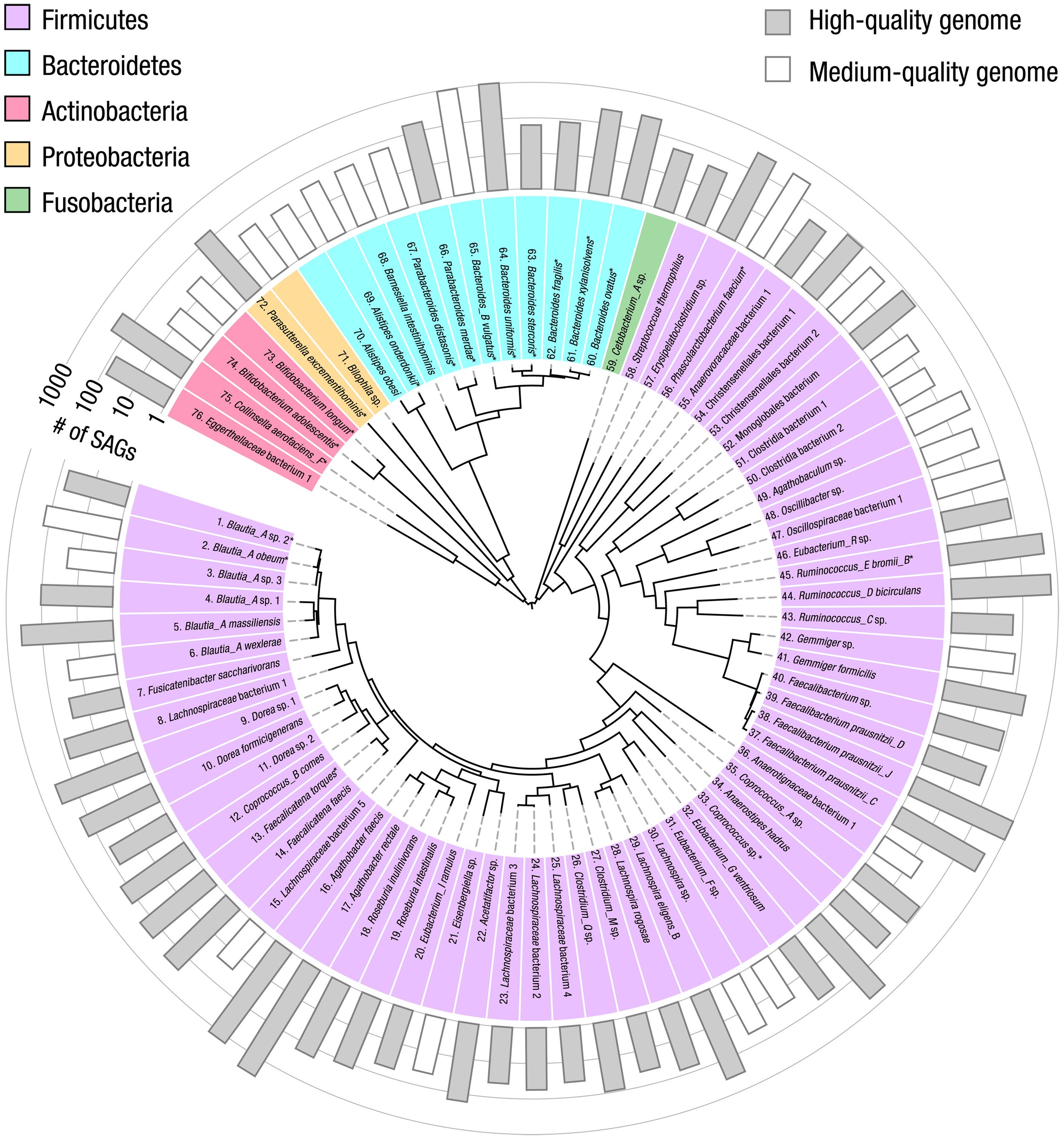
To determine whether each genome corresponds to a single species known to occur in the human gut microbiome, we compare each coassembled genome against a public database (GTDB-Tk) (59), using the ANI >95% criterion to identify matches of the same species. We obtain a broad mix of species from diverse phyla including Firmicutes, Bacteroidetes, Actinobacteria, Proteobacteria, and Fusobacteria (reported with assembly quality information in table S3). Several species well known in the human gut microbiome are abundant, including Faecalibacterium prausnitzii, Bacteroides uniformis, and B. vulgatus. For each of these 76 genomes, we list the name (colored according to corresponding phylum), illustrate its phylogenetic relationships with other species with a dendrogram, and indicate the number of SAGs used in its coassembly with the length of the outer bars, shaded for those of high quality, in Fig. 2.

Fig. 2. Coassembled genomes of 76 bacterial species in the human gut microbiome of a single human donor.

These 76 bacterial species have high- or medium-quality coassembled genomes. A phylogeny constructed from ribosomal protein sequences is represented by the dendrogram in the center of the circle. The phylum of each species is indicated by the background color behind each listed species name (GTDB-Tk database); the 19 species with genomes from isolates cultured from the same human donor are marked with an asterisk. The number of SAGs used for coassembly (abundance) is indicated by the bars in the outermost ring, shaded in gray for the 52 high-quality genomes and unshaded for the 24 medium-quality genomes.

Because there exists for these samples a large number of isolates cultured from the same human donor (12), we compare the coassembled genomes with the “gold standard” genomes derived from isolates. We find 19 species for which the coassembled genomes have corresponding isolate genomes, which we mark with an asterisk following each species name in Fig. 2. The ANI exceeds 99.5% in 17 species; these data provide strong evidence for the faithful reconstruction of genomes that closely match those of the cultured isolates, with low contamination.

With only a small set of culture-free experiments, we recover a broad set of accurate reference genomes from more species than those recovered from any other single gut microbiome. These genomes enable us to assign a large majority of single-microbe SAGs in the sample to one of these 76 species.

Microbial diversity in the human gut microbiome

Although species-level genomes provide one approach to assess microbiome diversity, the diversity of the human gut microbiome is typically assessed with metagenomics. We follow the spirit of this metagenomic approach and repurpose the droplet-based dataset to mimic that produced in metagenomics, by considering all reads from all SAGs in each sample. We classify each read in each sample by comparing it with the public database of microbial genomes (60); we also perform this comparison on each read from the corresponding metagenomic datasets (12). Each stool sample contains thousands of cells, in contrast to metagenomics which typically accumulates genomic data from millions of cells. Nevertheless, we recover 96.9 to 99.8% of the genera found by metagenomic analysis of the seven stool samples (figs. S3 and S4 and table S2).

The large collection of coassembled species-level genomes, however, provide an additional way to assess diversity with even greater precision at the species level. We align all metagenomic reads to the combined genome of all coassembled species irrespective of quality and find that 96 to 98% of these reads align, thereby providing further evidence that the droplet-based method does not miss any noticeable number of abundant taxa. For the 76 species with high- or medium-quality genome coassemblies, we estimate the relative abundance of each species in both metagenomics and the droplet-based approach. In metagenomics, the number of cells from a given species is proportional to the average read coverage over its genome; by contrast, in the droplet-based method we infer relative cell number by counting SAGs corresponding to the given species. We find that both abundance estimates are well correlated for the 76 species (fig. S5), though with one notable trend: In general, Gram-negative species—particularly those from Bacteroidetes and Proteobacteria—are underrepresented in the droplet-based method; by contrast, Gram-positive species, including Firmicutes and Actinobacteria, are overrepresented—albeit with a few exceptions (fig. S6). These trends may result from differences in lysis methods: for the metagenomics samples, we follow standard lysing protocols that use mechanical bead beating; because such mechanical methods have not been demonstrated in droplets, we use purely enzymatic methods known to favor Gram-positive species.

Strain-resolved genomes in the human gut microbiome

Many species in the human gut microbiome are represented by multiple strains (61); different strains may play distinct roles within complex microbial communities and express different sets of genes to carry out these roles (62). Linking specific genes and consequently their functionality to the strains which contain them requires knowledge of the genomes from those individual strains. Moreover, because each microbe inherently represents only a single strain, definitive identification of each SAG requires strain-resolved reference genomes.

To explore the possibility that the coassembled genomes contain contributions from more than a single strain, we further examine the comparison between the 19 coassembled genomes and cultured isolates of the same species; each of these isolates represents only a single strain. In general, the coassembled genome of a species with multiple strains contains some contigs specific to each strain; not all of these contigs appear in the single-strain genomes of the corresponding isolates. Consequently, we determine the shared genome fraction—the percentage of bases in each coassembled genome that are shared with isolate genomes from the same species. We find that for the comparison in 16 species, the shared genome fraction is above 96% and the ANI value exceeds 99.9%; these data suggest that each of these 16 coassembled genomes represents a single strain. By contrast, for the remaining three species, Blautia obeum, B. vulgatus , and Parasutterella excrementihominis, the shared genome fraction is far lower (between 70 and 90%) and ANI are all <99.6% (fig. S7). These lower values suggest that the genomes of these three species may include multiple strains or strains that do not appear among the cultured isolates. In principle, directly comparing all pairs of SAGs to estimate the fraction of their shared genomes could distinguish strains. However, the coverage of each SAG is expected to be <25% on average, for example 7% of the genome for B. vulgatus. This coverage suggests that such pairwise comparisons will not be reliable and instead motivates a different approach.

To distinguish strains, we develop a method that leverages the differences among homologous sequences between SAGs, specifically the single-nucleotide polymorphisms (SNPs). To illustrate this method we examine ~900 SAGs of B. vulgatus—the most abundant of the three species—and align reads from each SAG against the coassembled B. vulgatus genome, then identify ~12000 total SNP locations. For each SAG, we determine the SNP coverage, the fraction of all SNP locations in the genome that occur among the reads of that SAG; this SNP coverage is 8% on average, comparable to the average genome coverage. For each pair of SAGs, we measure the fraction of total SNP locations that occur in both and find this fraction to be ~0.7%, corresponding to ~80 SNPs, which is consistent with roughly the square of the SNP coverage. Microbes of the same strain have nearly identical genomes (12, 14) such that two SAGs representing the same strain almost always have the same base at each SNP location shared by both SAGs; conversely, SAGs representing different strains show considerably lower similarity (61). Inferring the similarity of the bases at shared SNP locations in each pair of SAGs is governed by a binomial process; therefore, the average of 80 SNPs in each SAG pair should be sufficient for a robust inference, with an uncertainty of 6% or less. Consequently, the comparison of SNPs provides a promising approach to determine strains.

To test this possibility, in all pairs of SAGs, we examine the bases at all shared SNP locations and determine the fraction of locations where both SAGs have the same base. To probe whether these SAGs fall into any distinct groups, we visualize the SNP similarity between all pairs of SAGs with dimensional reduction (63). Notably, we find that the SAGs fall into four clearly distinct clusters as shown in Fig. 3A. We independently validate the presence of these SAG groups with hierarchical clustering, which yields the same groupings with 99.8% overlap (fig. S8).

To test whether these clusters correlate with different strains, we examine the bases at SNP locations within each SAG cluster. We determine which base occurs most frequently at each SNP location; the set of these bases at each SNP location forms the consensus genotype of each SAG cluster. Then, for each SAG, we calculate the fraction of its SNPs that have the same base at the corresponding location in the consensus genotype of each of the four SAG clusters. Within each SAG cluster, we find that constituent SAGs share extremely high SNP similarity with the corresponding consensus genotype. For example, in the two clusters with the highest number of SAGs, almost all have the same base in >99% of the SNP locations as shown in the scatterplot and histograms in Fig. 3B. By contrast, SAG clusters show much lower overlap with the consensus genotypes of other clusters; for the two clusters with the highest number of SAGs, all SAGs in each cluster share fewer than 10% of the bases at SNP locations with the consensus genotype of the other cluster, as shown in the figure. These trends persist among the other clusters (fig. S8). Together, these results provide strong evidence that SAGs within these clusters represent the same strain.

To further examine whether these four clusters correspond to actual B. vulgatus strains, we coassemble the reads within each SAG cluster. We obtain high-quality genomes for the two groups with the most SAGs, which we label candidate strains A and B; one medium-quality genome, C; and one additional genome of lower quality, D (table S4). We compare these coassembled genomes with the genomes of two distinct B. vulgatus isolate strains cultured from the same human donor (12). We find that both isolate genomes have closely matching coassembled counterparts (A and C) with ANI values and shared genome fractions exceeding 99.9 and 97%, respectively, as shown in Fig. 3C. These high values are consistent with those that occur between genomes of the same strain, thereby providing strong evidence that these coassembled genomes each represent a single, genuine strain of B. vulgatus. Notably, the second-most populous cluster—candidate strain B, with several hundred SAGs—does not appear among the nearly one hundred isolates of B. vulgatus cultured from the same human donor (12). Together these results demonstrate the capabilities of this SNP-based approach to correctly identify both the major known strains of B. vulgatus and potential new strains that have not been cultured, while at the same time enabling the accurate coassembly of their genomes.

Fig. 3. Strain-resolved genomes of B. vulgatus in the human gut microbiome.

(A) Dimension-reduction (UMAP) visualization of B. vulgatus SAGs, based on comparison of their sequences at SNP locations. SAGs fall into four distinct, widely separated clusters; the symbol for each SAG is colored according to the cluster in which it is grouped. (B) Scatterplot and histograms illustrating the fraction of SNPs from each SAG that match consensus genotypes for SAGs in the two most abundant clusters, A and B. In almost all cases, each SAG shares the same base in more than 99% of the SNP locations in its corresponding consensus genotype; by contrast, the SNP overlap with the consensus genotype of the other cluster is much lower, typically 5% or less. The symbols in each cluster are colored as in (A). (C) Phylogeny of the coassembled high- and medium-quality genomes of B. vulgatus strains and comparison with the corresponding genomes of strains of isolates cultured from the same human donor. The horizontal axis of the dendrogram represents the ANI values between these strain-resolved genomes, demonstrating that coassembled strain C and isolate S1 are the same strain; similarly, coassembled strain A and isolate S2 are the same strain. By contrast, the second most-abundant strain, B, does not appear among the isolates cultured from the same human donor. (D) Relative abundance of the four B. vulgatus strains in the seven longitudinal samples.

We further apply this SNP-based analysis to the remaining species with high- or medium-quality species-level genomes. We find nine additional species with multiple strains and coassemble their genomes (fig. S9 and table S4). We compare the genotype of each SAG to its corresponding strain-resolved consensus genotype and observe that <1% of the SAGs have <95% similarity with the consensus genotype (fig. S10); these results are similar to those from B. vulgatus and provide strong confirmation that the separation of SAGs from different strains are robust. In total, we obtain 86 high- and medium-quality strain-resolved genomes from 76 species—from just one set of experiments—and compare to corresponding isolate genomes cultured from the same human donor. We find excellent agreement for B. obeum, with an ANI of 99.9% and shared genome fraction of 95%; this again confirms—just as in the case for B. vulgatus—that the coassembled genome represents a single, genuine strain (for the remaining multistrain species, we have no isolate genomes of the same strains with which to compare). Notably, we are able to achieve this accurate identification of strains and the coassembly of their genomes even with a level of coverage that yields an average of <100 shared SNP locations between all pairs of SAGs.

The capability to identify the strain of each individual SAG also enables us to follow the relative abundances of these strains over time in the human donor, giving insight on bacterial population dynamics. The abundances of these strains appear to shift only gradually throughout the year and a half over which samples were collected; for instance, we observe quite similar abundances in B. vulgatus in the two samples collected on successive days around day 400, as shown in Fig. 3D. These observations are consistent with previous studies showing that different Bacteroidetes species can colonize the human gut for decades stably, and that different strains of the same Bacteroidetes species can coexist with stable relative abundance (64).

The results demonstrate the capability of this approach to resolve subspecies strains and reconstruct their strain-resolved genomes, even when the SAGs have coverage of only ~10% of the genome. Furthermore, the droplet-based approach can obtain strain-resolved genomes from strains which have not been cultured; this is of particular importance in the human gut microbiome, where many strains are difficult to culture. Consequently, this method contributes a new way to examine the strain-resolved structure and dynamics of the genomic information within the human gut microbiome independent of the bias imposed by what has been cultured. These high-quality, strained-resolved genomes from a broad range of strains from the gut microbiome of a single human donor not only allow greater precision in the identification of a large majority of SAGs, but further enable the probing of broader genomic aspects of the microbial community, particularly those involving microbes of different strains.

HGT within the human gut microbiome

One particularly notable genomic aspect of microbial communities is how microbes exchange genetic information; one of the most well-known mechanisms is HGT, which is frequently observed within the human gut microbiome (20, 21, 65, 66). In general, the genomes of different bacterial species will differ considerably; however, one of the major indicators of HGT is a nearly identical sequence shared between genomes from different species (21, 67). The large number of strain-resolved genomes originating from the gut microbiome of a single human donor offers the potential to detect HGT by identifying the common sequences shared between specific microbial taxa.

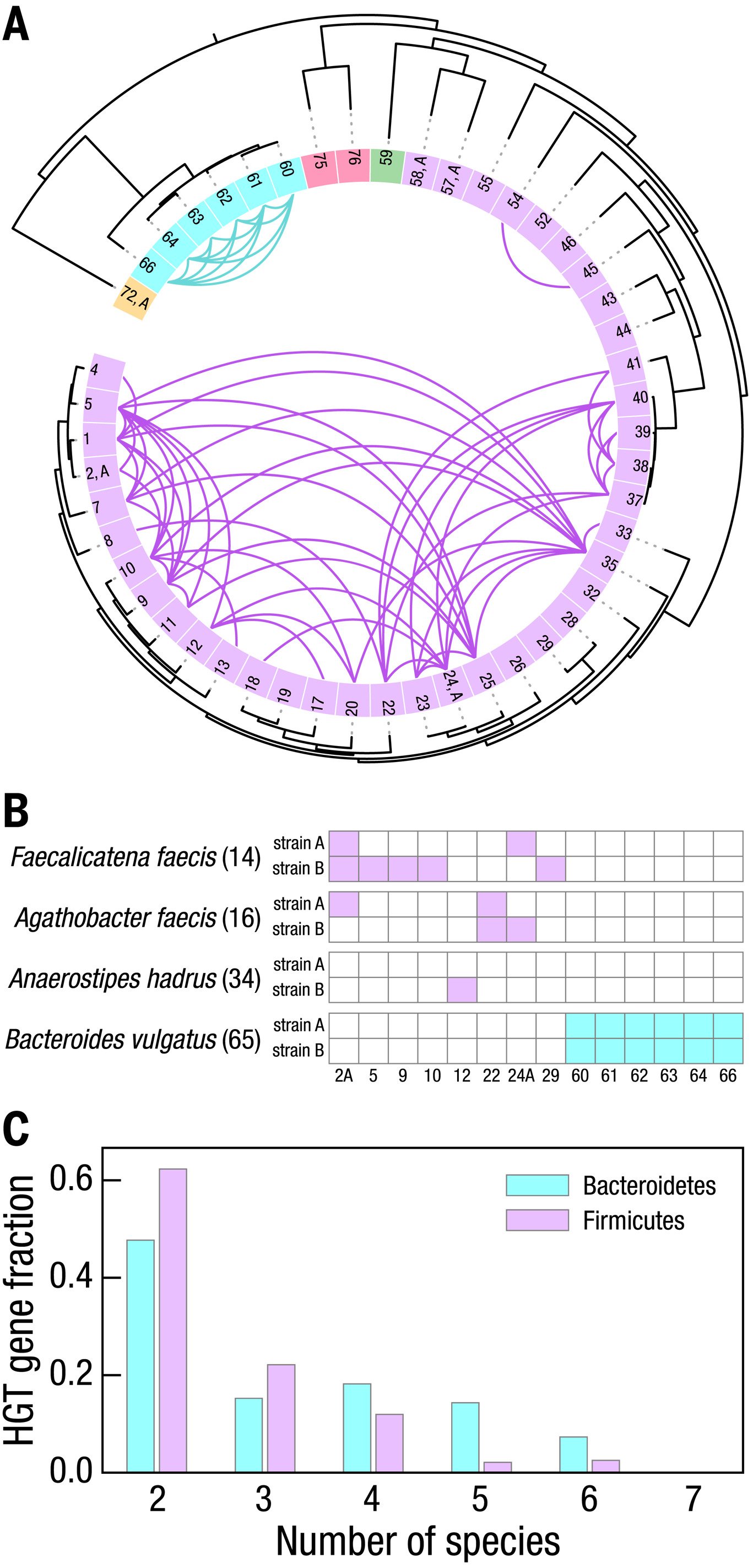
To explore this sequence matching approach, we designate an HGT event between genomes from two species as the presence of a common sequence of at least 5 kb with 99.98% similarity. We apply these criteria to all 57 high-quality strain-resolved genomes, filter out potential contamination due to SAG merging (fig. S11), and observe 265 HGT sequences between 90 pairs of strains from different species, which are all HGT events within the same phylum: 65 strain pairs are within Firmicutes and 25 are within Bacteroidetes.

To evaluate whether these events might be false positives caused by contamination, we align the reads from all SAGs of each species pair against each HGT sequence, and determine the fraction of all SAGs that have adequate coverage; under a null hypothesis that if an observed HGT event were in fact a result of contamination and the sequence was absent from one of the species, then only a small fraction of its corresponding SAGs would align to the HGT sequence with sufficient coverage. Instead, we find that all of the observed HGT sequences align to a number of SAGs considerably greater than that expected under the null hypothesis in both species of each pair, thereby confirming that there are no false positives (fig. S12). Furthermore, we examine the HGT sequences from the pairs of species with corresponding cultured isolates and find that 100% of the HGT sequences determined from the coassembled genomes occur in the isolate genomes of both species.

The HGT sequences we observe encode genes involved in a variety of metabolic, cellular, and informational functions (table S5); genes indicative of phage, plasmid, and other forms of mobile genetic elements exist in ~80% of the observed HGT sequences. Among the 49 species with a single high-quality strain, we observe 66 HGT events, as shown in Fig. 4A. Notably, among the species with multiple high-quality strains we observe that individual strains of Agathobacter faecis, Faecalicatena faecis, and Anaerostipes hadrus exchange genes with different Firmicutes species whereas both strains of B. vulgatus exchange genes only with the same six other Bacteroides species, as shown in Fig. 4B. Together, these data demonstrate the ability to resolve HGT to the level of individual strains.

To determine whether any of these HGT events involve more than two strains, we identify all of the genes that occur within HGT regions and count the number of strains whose HGT sequences contain each gene. We observe that approximately half of the genes are shared among three or more species, providing strong evidence that these HGT events emerged within this single human donor. Within Bacteroidetes, genes detected from HGT sequences are shared by an average of 3.2 strain-resolved genomes versus 2.6 strains within Firmicutes, as shown in Fig. 4C (table S6).

Notably, we find several genes that occur in the HGT sequences of six or seven Bacteroidetes strains. We examine the HGT sequences containing these particular genes and find that these sequences are connected with an integrative conjugative element containing a type VI secretion system (T6SS), consistent with previous analysis using cultured isolates of Bacteroides from the same human donor (14); T6SS is one of the most-studied systems in Bacteroides that mediates interstrain competition between Bacteroides strains and has been shown to transfer between members of the same microbiome. In Firmicutes, we also observe genes shared among HGT sequences of six different strains; these HGT sequences contain genes annotated as recombinase, suggestive of an integrative mobile element or prophage.

Fig. 4. HGT among bacterial strains within the human gut microbiome of a single donor.

(A) HGT among the 49 species with a single high-quality strain-resolved genome, following the order, numbers, and colors of Fig. 2. Detected HGT between two genomes indicated with a curve whose color matches that of the phylum of each species pair. (B) HGT between species with multiple high-quality strain-resolved genomes and species with single high-quality strain-resolved genomes, following the numbering in (A). For the bacteria in phylum Firmicutes (Agathobacter faecis, Faecalicatena faecis, and Anaerostipes hadrus), each strain has HGT with different sets of species. For the phylum Bacteroidetes, the only multistrain species is B. vulgatus, which has HGT between both of its strains and all other species in this phylum. (C) Distribution of the number of species in which HGT genes are shared. Approximately half of the genes in these HGT sequences are shared among more than two species; several genes occur in six or seven bacterial strains.

Together, these data provide strong evidence that our methodology detects HGT widely and robustly, among strains of many species from multiple phyla within the gut microbiome of a single human donor. The detection of HGT among six or more species within this single microbiome suggests that HGT may have important functional consequences to the recipient strains. These methods provide new tools to investigate the interactions of multiple microbes within the human gut microbiome.

Host-phage association in the human gut microbiome

The ability to investigate microbial interactions within the human gut microbiome is not limited to only bacteria, but also includes other types of microbes. Indeed, the diversity analysis reveals the presence of viruses—specifically crAssphage, the most abundant bacteriophage recognized at present from the human gut microbiome (68, 69). The general regulatory role of bacteriophages, thought to modulate the abundance and behavior of bacteria, is only beginning to be understood within complex microbial communities (70, 71). The droplet-based method encapsulates not only an individual bacterium but also any bacteriophages physically colocated with it, providing a direct means to probe host-phage association. To explore this association, we compare the reads in each SAG to the crAssphage genome; we find that a few dozen SAGs contain a substantial fraction of crAssphage-aligned reads. Moreover, many of these SAGs also contain a significant fraction of reads which do not align to the crAssphage genome but instead to bacterial taxa; we align these reads against the coassembled genomes of 76 species to identify which, if any, bacterial species might associate with crAssphage strain in this particular human donor.

Significantly, we find that 14 SAGs are associated with only one species, B. vulgatus (P value = 4 × 10−9, Fisher’s exact test) (table S7) and that no other species associates significantly with crAssphage, as shown in Fig. 5A. These data strongly suggest B. vulgatus as the in vivo host species for crAssphage in this human donor, consistent with previous evidence that crAssphage is likely to be associated with Bacteroides species (68, 72). The statistical significance of the association indicates that this is not a result of simple random coencapsulation.

Furthermore, the unambiguous assignment of each SAG to one of the multiple strains of B. vulgatus enables even more precise characterization of in vivo host-phage association to the level of specific bacterial strains. We find that 13 SAGs represent the single B. vulgatus strain A, the most abundant (P value = 3 × 10−11), as shown in Fig. 5B.

These data demonstrate the unique advantages of the droplet-based approach to establish accurate in vivo host-phage association not only for an individual species but even more precisely to a specific strain. We identify which bacterial strains interact with bacteriophages and which strains do not; the genomic differences between these strains provide preliminary data that may contribute to understanding of the molecular mechanisms underlying these host-phage interactions and their longitudinal dynamics in the human gut microbiome.

Fig. 5. Host-phage association with strain specificity in the human gut microbiome.

(A) Association between the bacteriophage crAssphage and bacterial species with high- or medium-quality genomes, with species numbers as in Fig. 2. All P values are calculated with one-sided Fisher’s exact test. The only bacterial species that is significantly associated with crAssphage is B. vulgatus. (B) Association between the four strains of B. vulgatus and crAssphage. Only one specific strain of B. vulgatus—the most abundant strain, A—is significantly associated with crAssphage.

Discussion

Using Microbe-seq, a high-throughput method combining experiment and computation for single-microbe genomics, we obtain—without culturing—the genomic information of tens of thousands of individual microbes and de novo coassemble the strain-resolved genomes from 76 species, a large fraction of which have not been cultured. This high-throughput microfluidics-based approach allows for more practical individual examination of a sufficient number of microbes to achieve these results, even with an average coverage of less than a quarter of the genome. The close agreement with strains for which we have corresponding cultured isolates confirms the accuracy of this approach. These strain-resolved genomes enable the reconstruction of an HGT network within a single human; when sampled over time, these data may allow the monitoring of microbe response, at the level of specific genes in specific strains, to selective pressures unique to that person, such as disease, diet, or antibiotic treatment. In addition, the in vivo association between specific strains of bacteriophages and bacteria could provide specific starting points to investigate how phages modulate microbial composition and possibly guide subsequent development of phage-based therapeutics.

Scaling up the analysis to examine an order of magnitude (or more) microbes from complex microbial communities would shed light on important questions without requiring any other qualitative changes to the existing procedures. In the human gut microbiome, sequencing hundreds of thousands of cells would likely allow for identification of nearly all of the present species and strains, thereby enabling far more accurate surveys of diversity and abundance. Moreover, expanding the present investigation to a larger population of humans could allow direct exploration of the effects on human health of key microbial pathways and genes, opening up potential directions for future therapeutic developments.

We envision several routes for further technical improvement. Integrating long-read sequencing technologies are likely to lengthen the coassembled contigs considerably, improving the quality and completeness of resulting genome assemblies (28). Exploring additional lysis conditions would improve the evenness and efficiency of lysis, potentially allowing investigation of microbes in other phyla or even other kingdoms such as fungi. Combining these methods with functional sorting, such as IgA bind-and-sort, would correlate functional outcomes with strain-level genomic information and single-cell resolution.

Microbe-seq provides a particularly effective and practical approach in a single laboratory-scale experiment to identify and sequence fully all of the major strains in microbial communities beyond the human gut microbiome, without any a priori knowledge of constituent microbes. The practical improvements provided by our methodology may make feasible the investigation of microbial communities that affect the environments, lives and health of human communities that otherwise lack access to the resources to even begin to investigate these effects.

Materials and methods

Experimental model and subject details

We obtain stool samples from OpenBiome, a nonprofit stool bank, under a protocol approved by the institutional review boards at MIT and the Broad Institute (IRB protocol ID # 1603506899). The subject is a healthy male, 28 years old at initial sampling, screened by OpenBiome to minimize the potential of carrying pathogens and de-identified before receipt of samples. We homogenize stool samples from this donor, mix with 25% glycerol, and freeze at −80°C. For each experiment, we wash 1-3 μL of stool sample in 1 mL 1X PBS three to five times and resuspend it in 1X PBS with 15% (v/v) Optiprep density gradient medium (Sigma-Aldrich D1556) as the microbial suspension.

Mock community

We culture four bacteria strains, Bacillus subtilis ATCC 6051-U, Escherichia coli ATCC 25922, Klebsiella pneumoniae ATCC 35657, and Staphylococcus aureus ATCC 6538 in 1 mL LB liquid medium (L3522 Sigma Aldrich) overnight. We wash each bacterial culture with 1 mL 1X PBS three to five times and resuspend bacteria in 1X PBS with 15% (v/v) Optiprep density gradient medium (Sigma-Aldrich D1556). We combine approximately the same volume of these four bacterial strains and dilute to a final concentration of 5-50 million microbes/mL.

Microfluidic device fabrication

We print the device designs (fig. S1) as photomasks (CAD/Art Services, Inc.), and fabricate devices according to well-established soft-lithography procedures (73). We use photolithography and the photomasks to transfer each device design to a silicon wafer with SU8 photoresist. We cast polydimethylsiloxane (PDMS) (Sylgard 184) on the SU8 structure, where the SU8 structure on silicon wafer serves as a master for replica molding. We bake at 65°C for at least 2 hours to cure the PDMS and delaminate the resulting PDMS replicas off the master. We seal with glass slides (Corning, 2947) to create the microfluidic devices and make their surfaces hydrophobic by flowing Aquapel (PGW Auto Glass, LLC) through the channels. We remove excess residual Aquapel by flowing compressed air in the channels of microfluidic devices and bake the devices at 65°C overnight.

Isolation and lysis

We isolate microbes by encapsulating them into droplets with lysis reagents using a microfluidic device (fig. S1A and movie S1). We put the microbial suspension in a 1 mL syringe (BD Luer-Lok 1-mL syringe, 309628) and connect the syringe to the microbial suspension device inlet via a needle (BD Precisionglide syringe needles, Z192384-100EA, Sigma Aldrich) and polyethylene tubing (BB31695-PE/2, Scientific Commodities, Inc.). We connect similarly the lysis reagents and oil, 2% (w/v) surfactant (RAN biotechnologies, 008-FluoroSurfactant) in HFE 7500 (3M), to the device. We use flow rates of 30 μL/h for the microbial suspension, 120 μL/h for lysis reagents, and 300 μL/h for the oil. We collect droplets from the device outlet into a PCR tube and replace the oil from the bottom with 100 μL of 5% (w/v) oil. We add 100 μL mineral oil (MI499, Spectrum Chemical MFG Corp.) on top of the emulsion to avoid the evaporation of the aqueous phase in the droplets. We remove most of the oil from the bottom of the tube and incubate to lyse the microbes inside droplets.

We prepare an 80 μL lysis reagent mix for each experiment: 10 μL green buffer (prepGEM Bacteria, PBA 0100), 1 μL lysozyme (prepGEM Bacteria, PBA 0100), 1 μL prepgem (prepGEM Bacteria, PBA 0100), 1 μL lysostaphin (1 mg/ml in 20 mM sodium acetate, pH 4.5, Sigma, L7386), 2 μL 20 mg/mL bovine serum albumin (BSA, B14, Thermofisher), 2 μL 10% tween-20 (diluted from Tween-20, Sigma-Aldrich, P9416-50mL), 1 μL 100 uM random hexamer with the last two 3′ end bases phosphorothioated (IDT), and 62 μL water.

The incubation program for lysis is: 37°C for 30 min, 75°C for 15 min, 95°C for 5 min and sample storage at 4°C.

Whole-genome amplification

We transfer the droplet emulsion to a syringe and reinject droplets into a microfluidic merger device (48) (fig. S1B and movies S2 and S3). In the same device, we use a separate droplet maker to form droplets that encapsulate multiple displacement amplification (MDA) reagents. We synchronize the frequency of sample droplet re-injection and reagent droplet-making to form droplet pairs. Applying electric fields of 50-200 V at a frequency of 25 KHz through a pair of electrodes, we merge each droplet pair to add MDA reagents. We use flow rates of 60 μL/h for sample droplets, 100 μL/h for 2% (w/v) oil (fig. S1B, label 2), 75 μL/h for MDA reagents, and 250 μL/h for 2% (w/v) oil (fig. S1B, label 4). We incubate to amplify microbial genomes.

We prepare a 100 μL MDA mix for each experiment: 16 μL 10X phi29 DNA Polymerase Buffer (Lucigen, 30221-1), 0.5-2 μL 100 uM random hexamer with last two 3′ end bases phosphorothioated (IDT), 0.8-3.2 μL 25 mM dNTPs (Thermo Fisher, R1121), 8 μL phi29 DNA Polymerase (Lucigen, 30221-1), 2 μL 20 mg/mL bovine serum albumin (BSA, B14, Thermofisher), and we add water to make the total volume to 100 μL.

The incubation program for MDA is: 30°C for 6-8 hours, 65°C for 10 min and sample storage at 4°C.

Tagmentation

We merge sample droplets with droplets containing commercially available tagmentation reagents (Nextera), utilizing a different droplet merger device (fig. S1C and movies S4 and S5). We use flow rates of 25 μL/h for sample droplets, 100 μL/h for 2% (w/v) oil (fig. S1C, label 2), 75 μL/h for tagmentation reagents, and 300 μL/h for 2% (w/v) oil (fig. S1C, label 4). We incubate to tagment these DNA products.

We prepare a 90 μL Nextera mix for each experiment: 60 μL TD Tagment DNA Buffer (Illumina, 15027866), 12 μL TDE1 Tagment DNA Enzyme (Illumina, 15027865), 1.8 μL 20 mg/mL bovine serum albumin (BSA, B14, Thermofisher), 1.8 μL 10% tween-20 (diluted in water from Tween-20, Sigma-Aldrich, P9416-50mL), and 14.4 μL water.

The incubation program for tagmentation is: 55°C for 10 min, and sample storage at 10°C.

Bead synthesis

We synthesize beads used for combinatorial barcoding by adopting a previously reported method (44, 74). In brief, we make droplets containing acrydite-modified DNA oligos using a photo-cleavable linker (table S8, Hydrogel DNA primer, IDT) and acrylamide:bisacrylamide solution. We keep these droplets at 65°C overnight to polymerize them into uniform soft gel beads covalently bonded to the DNA oligos by photo-cleavable linkers. We extend DNA oligos on beads enzymatically with a two-step split-and-pool synthesis protocol to prepare beads with a diverse barcode sequence library. At the first split-and-pool synthesis step, we evenly split beads into a 96-well plate where each well contains a unique barcode-1 oligo (table S8, IDT). We anneal these oligos with hydrogel oligos and extend them with Bst 2.0 DNA polymerase (M0537L, NEB). After the first split-and-pool synthesis step, we pool beads, wash them and evenly split them into a 384-well plate where each well contains a unique barcode-2 oligo (table S8, IDT). We perform the second barcode strand synthesis in the same way as we extend the first barcode strand. We avoid exposing beads to strong light.

Each soft gel bead has millions of primers with the same sequence. Each full sequence contains two barcode regions: the first region has a diversity of 96; the second region, 384. Overall, the barcoding bead library has 36864 (96×384) possible sequences.

Bead preparation for barcoding

We wash 200 μL of beads with 1 mL bead wash buffer (10 mM pH 8.0 Tris-HCl, 0.1 mM EDTA and 0.1% (v/v) Tween-20), three times in a tube. We withdraw supernatant from the top, leaving 500 μL in the tube. We add 300 μL water and 200 μL 5X Phusion HF detergent-free buffer (F520L, Thermo Fisher) to the tube. We vortex the beads and keep them at room temperature for 1 min. We centrifuge beads, remove supernatants, and use these beads for barcoding.

Barcoding

We merge sample droplets with droplets containing PCR reagents and a barcoding bead, using a droplet-merger microfluidic device (fig. S1D and movies S6 to S8). We use flow rates of 50 μL/h for sample droplets, 100 μL/h for 2% (w/v) oil (fig. S1D, label 2), 15-25 μL/h for beads, 140 μL/h for PCR reagents, and 400 μL/h for 2% (w/v) oil (fig. S1D, label 5). We release barcode oligos from beads by exposing droplets to UV light (365 nm at ~10 mW/cm2, BlackRay Xenon Lamp) for 10 min. We perform PCR to barcode the DNA in the droplets.

We prepare a 240 μL PCR mix for each experiment: 136 μL water, 68 μL 5X Phusion HF detergent-free Buffer (F520L, Thermo Fisher), 8 μl 10 mM dNTPs (diluted from 25 mM dNTP mix, Thermo Fisher, R1121), 16 μl 10 μM RNS primer (table S8, IDT), 4 μl Phusion high-fidelity DNA polymerase (F530L, Thermo Fisher), 4 μl 20 mg/mL bovine serum albumin (BSA, B14, Thermofisher), 4 μl 10% tween-20 (diluted from Tween-20, Sigma-Aldrich, P9416-50mL).

The incubation program for barcoding is: 72°C for 4 min, 98°C for 30 s; 10 cycles of 98°C for 7 s, 60°C for 30 s and 72°C for 40 s; 72°C for 5 min, and sample storage at 4°C. We use slow ramping of 2°C/s at this step.

We observe the merger of some droplets after PCR, possibly during the high-temperature stage of PCR; such larger droplets may contain DNA from multiple microbes. We remove most of these droplets with droplet-size filter microfluidic device (75) (fig. S1E, movies S9 and S10) with flow rates of 120 μL/h for sample droplets and 2 mL/h for 2% (w/v) oil.

Droplet pooling and sequencing library preparation

We break the emulsion of droplets by adding 200 μL 20% (v/v) PFO (1H,1H,2H,2H-Perfluoro-1-octanol, 370533 Sigma Aldrich) in HFE 7500 (3M) into each sample after PCR. We purify the aqueous phase with 1.1X volume AMPure beads (A63881, Beckman Coulter) and resuspend into 32 μL DNA suspension buffer (10 mM pH 8.0 Tris-HCl and 0.1 mM EDTA). We use PCR to add sequencing adapters for sequencing (Illumina) and a sample index (Nextera index) to each purified DNA sample so we can sequence multiple samples in one sequencing run.

We prepare a 50 μL PCR mix for each experiment: 2.5 μL water, 10 μL 5X Phusion HF detergent-free Buffer (F520L, Thermo Fisher), 1 μl 10 mM dNTPs (diluted from 25 mM dNTP mix, Thermo Fisher, R1121), 2 μL 10 uM P5PE1 primer (table S8, IDT), 2 μL Nextera i7 primer (Illumina), 0.5 μl Phusion high-fidelity DNA polymerase (F530L, Thermo Fisher), and 32 μL DNA sample in DNA suspension buffer.

The incubation program for PCR is: 98°C for 30 s; 5-10 cycles of 98°C for 7 s, 60°C for 30 s, and 72°C for 40 s; in the end, 72°C for 5 min and sample storage at 4°C.

We purify samples with 0.8X volume AMPure beads (A63881, Beckman Coulter) and resuspend DNA products into 20 μL DNA suspension buffer (10 mM pH 8.0 Tris-HCl and 0.1 mM EDTA). We store these products at -20°C before sequencing.

Illumina sequencing

We sequence at depths ranging between ten thousand and two hundred thousand reads for each microbe. A custom read-1 primer (table S8, IDT) is required for the sample to be sequenced. For a 100 base-pair (bp) sequencing run, we use the following sequencing length configurations: read-1 sequence: 45 bp, which contains the barcode sequence; index-1 sequence: 8 bp; read-2 sequence: remainder, which contains the microbial sequence. For a 300 bp sequencing run, we use the following sequencing length configurations: read-1 sequence: 150 bp, the first 45 bp are barcode sequences, the last 75 bp are microbial sequences, and those in the middle are adapter sequences; index-1 sequence: 8 bp; read-2 sequence: remainder, which contains the microbial sequence.

Preprocessing of raw sequencing data

We group raw sequencing reads based on the 36864 barcodes, excluding barcodes associated with too few reads (~15% of total reads) and those with significantly more reads than other barcodes likely due to droplet merging (~5% of total reads). For the remaining barcodes, we designate the collection of microbial sequences associated with a single barcode as a single amplified genome (SAG). We use Trimmomatic (76) (version 0.36, LEADING:25 TRAILING:3 SLIDINGWINDOW:4:20 MINLEN:30) to remove low-quality reads and adapter sequences from each SAG for following analysis.

Mock sample alignment, quality assessment, and coverage

We use Bowtie2 (52) (version 2.2.6, default parameters) to align reads from each SAG to the combined genome of the four reference genomes (RefSeq: GCF_002055965.1, GCF_004151095.1, GCF_001936035.1, GCF_002025145.1), which reports the best hit of each read. We use SAMtools (77) (version 1.9) to check the number of reads that align to each of the four genomes and to calculate the purity of each SAG. For each SAG with high purity (>0.95), we align its reads to the most-aligned reference genome to determine its genome coverage.

Genome coassembly of microbial species in the human gut microbiome

We use SPAdes (53) (version 3.13.0,–sc–careful) to de novo assemble genomes from the reads of each of the 21914 SAGs. We compute and compare signatures of these assembled genomes using sourmash (78) (version 2.0, k-mer 51, default setting), which produces a matrix of estimated similarities between genomes. We use a hierarchical clustering method (SciPy version 1.1.0, method: complete, metric: Euclidean, criterion: “inconsistent”, and threshold: 0.95) to group SAGs into bins. We verify 0.95 as a threshold using mock samples. This set of parameters groups bins conservatively, minimizing the improper grouping of SAGs from different species. We use all the reads within each bin to coassemble a tentative genome, compare tentative genome similarities, and cluster the bins. We iterate this process until more than 10% of the assembled genomes have more than 10% contamination (estimated by CheckM version 1.0.13, default parameters) (56), which implies false clustering of SAGs; through four rounds, we group the 21914 SAGs into 364 bins.

To split bins that might contain SAGs from multiple species, we examine contig alignment patterns. Within each of the 364 bins, we align reads from each SAG to the de novo coassembled genome from that bin using bowtie2 (52) (default parameters). For each contig in the tentative genome with more than 1000 bp, we construct a vector for each contig with the number of reads aligned to the contigs from each SAG. We use a hierarchical clustering method (method: ward, default parameters) to group vectors of contigs into two groups. For each SAG, if >95% aligned reads are aligned to one of the two groups of contigs, it is designated as a SAG associated with that group of contigs. We assume that the remaining SAGs are a mixture of multiple species and exclude them from further analysis. We iterate this binary splitting process until we exclude more than 60% of the SAGs in the current bin, or both resulting new bins have fewer than 10 SAGs, or the change between the resulting new bin and the current bin is fewer than three SAGs. Using this process, we obtain 400 bins whose constituent SAGs we expect to represent a single species, with minimal contamination.

To combine bins of the same species for genome assembly, we use fastANI (55) (version 1.2, default parameters) to calculate average nucleotide identity (ANI) between all pairs of these 400 bins. Applying the commonly used ANI > 95% threshold, above which two genomes are considered to represent the same species, we generate 234 new species-level bins. We de novo assemble reads from all SAGs within each of these 234 bins and remove contigs shorter than 500 bp. To further eliminate contigs that may originate from other species within each genome, e.g., as a result of random contamination in individual SAGs, we fit a normal distribution with the coverage of contigs on a log scale and remove those contigs with coverages that are more than two standard deviations away from the mean of the distribution.

Among these 234 genomes, 76 genomes are of high-quality (>90% completeness and <5% contamination) or medium-quality (>50% completeness and <10% contamination), as assessed by CheckM (56) (default parameters). We use fastANI (55) (default parameters) to compare the genomes of these 76 bins to all microbial genomes (RefSeq as of September 2019), and to the published collection of more than a thousand cultured-isolate whole genomes (12). We identify the closest corresponding species-level genomes with ANI > 95% in both databases. The closest genomes in RefSeq to species Alistipes onderdonkii, Bacteroides fragilis, and Bacteroides ovatus are cultured isolate whole genomes from the same donor, reported previously (79); we exclude these three genome pairs from the ANI and shared genome fraction analysis (fig. S7). We use BLASTn (BLAST+, version 2.10.0) (80) (default parameters) to compare overlapping sequences between genome pairs.

The names of the species-level genomes in RefSeq are not always labeled consistently; for example, we have four species that are named as Blautia obeum in RefSeq, though their ANI values are less than 95%. We use both GTDB-Tk (59) (version 1.0.2, reference data version r89) and comparison to RefSeq genomes (as of September 2019) to assign taxonomies to all species. In the main text, we use taxonomies classified with GTDB-Tk and remove subgenus names, such as “A”.

Phylogeny analysis of genomes

To construct the phylogeny of the 76 species with high-quality or medium-quality genomes, we extract amino acid sequences of six ribosomal proteins (Ribosomal_L1, Ribosomal_L2, Ribosomal_L3, Ribosomal_L4, Ribosomal_L5, and Ribosomal_L6), concatenate and align them with Anvi’o (version 6.1) (81). We construct a maximum likelihood tree with RaxML (82) (version 8.2.12, standard LG model, 100 rapid bootstrapping). We use iTOL (version 5.5) (83) to visualize and annotate the resulting dendrograms.

Diversity of the human gut microbiome samples

For each of the seven samples, we temporarily ignore the barcode information and combine all reads from all SAGs from the sample. We use Kraken2 (84) (version 2.0.8, default parameters) to classify reads from each Microbe-seq dataset and corresponding metagenomic dataset (12) (standard Kraken database as of April 2019). For the analysis shown in fig. S4, we keep only the reads classified to a specific genus and use only this genus-level information for the comparison; similar analyses using all operational taxonomic units (OTUs) show similar results (table S2). For each metagenomic dataset, we align reads to the combined genome coassemblies from the 364 bins, irrespective of whether the bin is species level. Metagenomic reads are first quality filtered with fastp (version 0.12.4, parameters: -f 15 -t 15 -q 36 -u 10) and then aligned to the combined genomes using bowtie2 (parameter:–very-sensitive-local). We obtained overall alignment rates of 98.26%, 98.74%, 98.63%, 96.65%, 96.63%, 96.11%, and 98.64% for each of the seven metagenomic samples.

Abundance bias between Microbe-seq and metagenomics

We compare relative abundance from the 76 species with high- or medium-quality genome coassemblies. We estimate the cell number for each species in the metagenomic dataset by aligning metagenomic reads to each species-level reference genome and computing the average sequencing depth between the 20th and 80th percentiles in genome-wide sequencing depth. We infer cell number in the Microbe-seq dataset by counting the number of SAGs that we assign to each species; we normalize this cell-number inference across all these species and average across the seven longitudinal samples to obtain a single relative abundance inference for all species.

Differentiating strains of the same species

We use B. vulgatus as an example in the main text to illustrate the strain differentiation workflow; we use the same computational pipeline for all other species, without changing parameters, to resolve their constituent strains. The uncertainty in similarity of the bases at shared SNP locations in each pair of SAGs is the standard deviation of the normal approximation of the binomial distribution: uncertainty = sqrt[p(1−p)/n], where p is the probability of the event and n is the number of events. In the case of B. vulgatus, n=80 and the uncertainty is <6%.

Within each of the species with high- or medium-quality species-level genomes, we align (52) each SAG to the assembled genome. We use bcftools (77) (mpileup, filters: snps and %QUAL>30) to identify high-quality single-nucleotide polymorphism (SNP) mutations. We designate a SAG with fewer than 2 reads aligned to a SNP, as well as fewer than 99% of its reads being the same at a SNP as unknown/unaligned at this location. We remove SNPs with fewer than 5% of SAGs aligned to the location, and SNPs with fewer than two SAGs being the reference allele or fewer than two SAGs being the mutation allele. We also remove any SNP with fewer than 1% SAGs being the reference allele or fewer than 1% SAGs being the mutation allele. We remove any SAG that covers less than 1% or fewer than 10 of the kept SNP locations.

We identify thousands of SNP locations and remove up to 6% of SAGs. We construct a SNP vector to represent the base identity sequence of each SAG at each SNP location. To identify the number of strains of the species in the samples, we build a dendrogram of SAGs with hierarchical clustering (method: “ward”) using the SNP vectors of all SAGs. Although the number of clusters is not obvious from the dendrogram, we obtain a sequence of SAGs; in this sequence, SAGs with similar SNP sequences are closer. We compare similarities of SNP vectors between SAGs at their shared SNP locations and construct a similarity heatmap with SAGs ordered in the same sequence as the corresponding dendrogram. We observe block-diagonal squares in the heatmap, which indicates that SAGs within each square are closer to each other than to SAGs in other squares. Using the block-diagonal squares in the heatmap, we determine the number of strains, though this number is challenging to determine accurately for species with relatively few SAGS (<200) and for species with potentially more than two strains. For Blautia obeum, it is unclear whether there are 3 or 4 strains in the sample; for Parasutterella excrementihominis, it is unclear whether there are 2 or 3 strains. We apply UMAP (63) (default parameters) to the SNP data to create dimensional-reduction plots (fig. S9).

To remove SAGs that have reads from microbes of multiple strains, we construct the consensus genotype of each strain by comparing the SNP vectors of SAGs of the same strain. If more than 90% of the values at a SNP location from all SAGs within the strain are the same, we use the value for this SNP in the consensus genotype for the strain; otherwise we drop this SNP location for this strain. We compare the SNP vector of each SAG to the consensus genotype of each strain and assign strains to those SAGs that match more than 95% locations at the consensus genotype of only one strain, which excludes fewer than about 1% of the SAGs from each species. We coassemble strain-resolved genomes with reads from all SAGs in each of these assigned strains with SPAdes (53) using default parameters.

Horizontal gene transfer analysis

We detect HGT events by searching for blocks of DNA sequences shared by a pair of strain-resolved genomes that are longer than 5000 bp and more than 99.98% identical (14, 67). Assuming that species from the gut microbiome evolve with a molecular clock of 1 SNP/genome/year and that typical genome size is 5,000,000 bp, this set of criterion detects sequences that diverged within the past 1000 years and the HGT events likely emerged within the human host, based on known mutation rates (14). To filter out HGT sequences resulting from contaminated SAGs, we select all SAGs from each strain-resolved genome, and align reads from each SAG to the corresponding strain-resolved genome. We remove SAGs with an overall sequence alignment ratio below 90%, which eliminates three HGT sequences from two genome pairs, as no SAGs from one of the strain-resolved genomes have reads that cover the HGT sequences.

To further validate the remaining detected HGT sequences, we align reads from all the filtered SAGs from both HGT-associated species. We calculate the number of SAGs belonging to each strain-resolved genome with more than 500 bp coverage over the HGT sequence. We explore the statistical likelihood of the observed fraction of SAGs containing reads covering the HGT sequence. We build a null model that if we detect an artifactual HGT event between species A and B, that sequence actually only exists in the genome of species B, but appears in the SAGs of species A as a result of contamination. We assume a worse-than-real scenario that if a SAG from species A is contaminated by species B, this SAG will contain reads covering the false HGT sequence. We also assume a worse-than-real contamination rate of 20% SAGs for any strain and species. Under these assumptions, the upper limit for the probability that any SAG from species A is contaminated by B is: 20% × (relative abundance of B) = 0.2 × Nb / N, where Nb is the number of SAGs from species B, and N is the total number of SAGs. If the observed SAG number for species A is Na, and the observed number of SAGs contaminated by B is up to x, then the probability that equal or more than x of the SAGs from species A are contaminated by species B is 1-binom.cdf(x, Na, 0.2×Nb/N); this calculated quantity represents the upper limit of the P value for the observed fraction of SAGs containing reads from the HGT sequences.

To explore whether these HGT events either emerged within this human subject or before both strains colonized the host, we compare our results to the baseline detectable HGT from strains that are not from the same human host. For 39 species that we find a corresponding high-quality genome assembly from the NCBI database, we select the single genome that most closely matches the strain-resolved genome from Microbe-seq using ANI. We apply our exact HGT criteria to this collection of 39 genomes from the NCBI database, and compare with the corresponding 39 strain-resolved genomes from Microbe-seq in fig. S13.

We predict genes (open reading frames, ORFs) from the HGT sequences using prokka (85), (version 1.12, default parameters). We annotate ORFs using eggnog-mapper (86) (version 3.0, parameter: -m diamond–tax_scope auto–go_evidence nonelectronic–target_orthologs all–seed_ortholog_evalue 0.001–seed_ortholog_score 60–query-cover 20–subject-cover 0). For each HGT sequence, we assign the sequence to a certain type of mobile element if ORF annotations contain signatures of mobile elements (detailed information in table S5). To examine how many species share the same HGT sequences, we cluster all the ORFs from all HGT sequences using CD-HIT (87) (version 4.7, 100% similarity). For each gene cluster, we count the number of species whose HGT sequences contain genes within the gene cluster (Fig. 4C and table S6). We cluster genes from only the HGT regions and the HGT sequences detected via our method, which are likely incomplete fragments of the original HGT events; therefore, the number of species we report for each gene is likely an underestimation.

Host-phage association analysis

To identify SAGs that are associated with both crAssphage and a bacterial cell, we use bowtie2 (52) (default parameters) to align reads in each SAG to the crAssphage genome (Refseq: GCF_000922395.1). We designate SAGs with more than 5% reads aligned to the crAssphage genome as containing significant crAssphage reads (raising this threshold to 10% of reads yields the same result); we align the non-crAssphage reads of these SAGs to each of the 76 high- or medium-quality genomes, as well as the combined genome of these 76 genomes. We define purity of these SAGs as the maximum number of reads aligned to individual genomes divided by the number of reads aligned to the combined genome. We identify SAGs with more than 50% of reads aligned to one of these 76 genomes, and with purity of more than 95%. We designate the species of the SAG as the species of the most aligned genome. We count the number of SAGs assigned to each species and perform the “one species versus remaining species” one-sided Fisher’s exact test.

Acknowledgments

We thank members of the Weitz and Alm laboratories for helpful discussions and Y. Cai, W. Chen, Z. Cheng, N. Cui, L. Dai, R. Ding, P. Ellis, Z. Ge, J. Gong, H. Li, F. Ling, B. Liu, H. Liu, H. Pei, R. Rosenthal, J. Tang, Y. Wang, J. Xia, Y. Yao, X. Yu, Z. Zhang, Z. Zhang, and Z. Zhao for general discussions and comments on the manuscript. P.J.L. acknowledges support from the Massachusetts DTA through the SNAP and HIP programs. We thank OpenBiome for providing stool samples. We thank the MIT Center for Microbiome Informatics and Therapeutics and The Bauer Core Facility at Harvard University for providing sequencing services.

Funding: This work was supported by the following: US Department of Energy, Office of Science, Office of Biological & Environmental Research, grant DE-AC02-05CH11231 at Lawrence Berkeley National Laboratory by ENIGMA-Ecosystems and Networks Integrated with Genes and Molecular Assemblies; The National Science Foundation grant DMR-1708729; The National Science Foundation grant, through the Harvard University Materials Research Science and Engineering Center, DMR-2011754; National Institutes of Health grant P01HL120839; National Institutes of Health grant R21AI125990; National Institutes of Health grant R21AI128623; National Institutes of Health grant R01AI153156; National Aeronautics and Space Administration grant NNX13AQ48G; National Aeronautics and Space Administration grant 80NSSC19K0598.

Author contributions: W.Z., S.Z., H.Z., P.J.L., E.J.A., and D.A.W. conceived and designed the methodology; W.Z. developed and performed the experiments with assistance from S.Z.; S.Z., W.Z., Y.Y., D.M.N., and C.L.D. performed the data analysis with input from all authors; P.J.L., W.Z., and S.Z. wrote the initial manuscript; D.A.W., P.J.L., W.Z., S.Z., and E.J.A. revised the manuscript; all authors read and commented on the manuscript; E.J.A. and D.A.W. supervised the study.

Competing interests: E.J.A. is affiliated with Finch Therapeutics and Biobot Analytics. All other authors declare no other competing interests.

Data and materials availability: Combined fastq files for each stool sample, with read header containing the unique SAG ID and adaptor removed and filtered for quality, are available from NCBI Sequence Read Archive (Bioproject: PRJNA803937). Metagenomic fastq files are available from the previous publication (Biopoject: PRJNA544527). Commented scripts, intermediary data, and genome coassemblies are available at (88).

License information: Copyright © 2022 the authors, some rights reserved; exclusive licensee American Association for the Advancement of Science. No claim to original US government works. https://www.sciencemag.org/about/science-licenses-journal-article-reuse

The UGT2A1/UGT2A2 locus is associated with COVID-19-related loss of smell or taste

Scientists have discovered why specific individuals, including 1.6 million Americans to date, have significantly lost their sense of smell or taste due to coronavirus infections. Researchers have now studied the genes of nearly 70,000 individuals to uncover the loci involved.

This study was made possible because millions of people (none in my family) have given their money, DNA, and consent to 23andMe. Many of the same people that say they don’t want to be “part of an experiment” have certainly been part of many genetic studies as the fine print in the test kit allows the sale of the genetic information gleaned from each participant.

SARS-CoV-2 damages the sustentacular cells, the cells responsible for supporting olfactory neurons and signal transduction “processing odorants by endocytosing the odorant-binding protein complex, detoxifying, maintaining the cilia of mature olfactory receptor neurons and maintaining epithelial integrity.”

The genes highlighted in this study are GT2A1 and UGT2A2 encoding for enzymes that work to “digest” molecules for sensory processing.

As the wise Dr. Ron Evans of the National Academy of Scientists told me in 2005, “It is all about enzymes.”

The entire article published this month in Nature Genetics, is below and linked here.

AUTHORS: Janie F. Shelton, Anjali J. Shastri, Kipper Fletez-Brant, The 23andMe COVID-19 Team, Stella Aslibekyan & Adam Auton

Abstract

Using online surveys, we collected data regarding COVID-19-related loss of smell or taste from 69,841 individuals. We performed a multi-ancestry genome-wide association study and identified a genome-wide significant locus in the vicinity of the UGT2A1 and UGT2A2 genes. Both genes are expressed in the olfactory epithelium and play a role in metabolizing odorants. These findings provide a genetic link to the biological mechanisms underlying COVID-19-related loss of smell or taste.

Main

Loss of sense of smell (anosmia) or taste (ageusia) are distinctive symptoms of COVID-19 and are among the earliest and most often reported indicators of the acute phase of SARS-CoV-2 infection. It is notable from other viral symptoms in its sudden onset and the absence of mucosal blockage1. While a large fraction of COVID-19 patients report loss of smell or taste, the underlying mechanism is unclear2. In this study, we conducted a genome-wide association study (GWAS) of COVID-19-related loss of smell or taste, having collected self-reported data from over 1 million 23andMe research participants as described previously3. By asking study participants to report the symptoms they encountered during their COVID-19 experience, we identified SARS-CoV-2 test-positive individuals who reported a loss of smell or taste and contrasted them with test-positive individuals who did not report a loss of smell or taste.

Of the individuals who self-reported having received a SARS-CoV-2 positive test, 68% reported loss of smell or taste as a symptom (47,298 out of a total of 69,841 individuals). Female respondents were more likely than male respondents to report this symptom (72% versus 61%; chi-squared test, P = 5.7 × 10−178) and those with this symptom were typically younger than those without this symptom (mean age of 41 years for those with loss of smell or taste versus 45 years for those without; P = 2.34 × 10−199, Welch’s t-test). Among genetically determined ancestral groups, rates of loss of smell or taste ranged between 63% and 70% (Table 1). As expected, compared to other symptoms surveyed, loss of smell or taste was much more common among those with a SARS-CoV-2 positive test compared to those who self-reported other cold or flu-like symptoms but who tested negative for SARS-CoV-2 (Extended Data Fig. 1). In a logistic regression model predicting loss of smell or taste as a function of age, sex and genetic ancestry, individuals of East Asian or African American ancestry were significantly less likely to report loss of smell or taste (odds ratio (OR) = 0.8 and 0.88, respectively) relative to individuals of European ancestry (Supplementary Table 1).

For unrelated individuals with complete data, we conducted GWAS within each ancestry group separately (total sample size = 56,373) before performing a multi-ancestry meta-analysis using a fixed effects model. Each input GWAS was adjusted for inflation via genomic control (λ = 1.029, 1.037, 1.024, 1.042 and 1.071 within the European, Latino, African American, East Asian and South Asian ancestry GWAS, respectively), as was the subsequent meta-analysis (λ = 1.001). Within the multi-ancestry meta-analysis, we identified a single associated locus at chr4q13.3 (Fig. 1). No other locus achieved genome-wide significance in the multi-ancestry meta-analysis or in any of the input populations. The index SNP at this locus was rs7688383 (C/T, with T being the risk allele, P = 1.4 × 10−14, OR = 1.11). While most of the support for this genetic association within the multi-ancestry analysis comes from the European population (for which we have the largest sample size), the estimated effect sizes are consistent across populations (Supplementary Table 2). The credible set from the multi-ancestry analysis contained 28 variants covering a 44.6-kilobase (kb) region (chr4:69.57–69.62 megabases (Mb); Supplementary Table 3).

a, Manhattan plot. SNPs achieving genome-wide significance are highlighted in red. The nearest gene to the index SNP is indicated above the relevant association peak. b, Regional plot around the UGT2A1/UGT2A2 locus. The colors indicate the strength of linkage disequilibrium (r2) relative to the index SNP (rs7688383). Imputed variants are indicated with ‘+’ symbols; coding variants are indicated with ‘x’ symbols. Where imputed variants were not available, directly genotyped variants are indicated by ‘o’ symbols; coding variants are indicated by diamond symbol

Methods

Overview of study recruitment and data collection

Participants in this study were recruited from the customer base of 23andMe, a personal genetics company. Participants provided informed consent and participated in the research online, under a protocol approved by the external Association for the Accreditation of Human Research Protection Programs-accredited institutional review board, Ethical and Independent Review Services. Participants were included in the analysis based on consent status as checked at the time data analyses were initiated.

Full details of the data collection paradigm for this study have been described previously3. In brief, primary recruitment was carried out by email to approximately 6.7 million 23andMe research participants over 18 years of age and living in the USA or UK. Additionally, pre-existing customers were invited to participate in the study through promotional materials on the 23andMe website, the 23andMe mobile application and via social media. Study participation consisted solely of web-based surveys, including an initial baseline survey and three follow-up surveys fielded each month after completion of the baseline survey. The surveys collected information regarding individuals’ experiences with COVID-19 and included questions regarding recently experienced symptoms with or without a SARS-CoV-2 positive test. Enrollment continued after the initial recruitment efforts until a data freeze was taken for this study in March 2021, when 1.3 million participants had completed the baseline survey.

Phenotype definition for GWAS

Using the information derived from the surveys, we defined a phenotype to contrast SARS-CoV-2 positive individuals that experienced COVID-19-related loss of smell or taste from those who did not. Specifically, participants were asked to respond to the question ‘Have you been tested for COVID-19 (coronavirus)?’, with possible responses ‘Yes, it was positive/Yes, it was negative/No/My results are pending/I’m not sure’. Of those who responded ‘Yes, it was positive’, we further considered the question ‘During your illness, did you experience any of the following symptoms?’, to which participants could select as many as needed from the following list of responses: ‘Muscle or body aches/Fatigue/Dry cough/Sore throat/Coughing up of sputum or phlegm (productive cough)/Loss of smell or taste/Chills/Difficulty breathing or shortness of breath/Pressure or tightness in upper chest/Diarrhea/Nausea or vomiting/Sneezing/Loss of appetite/Runny nose/Headache/Intensely red or watery eyes’. We defined cases as SARS-CoV-2 test-positive individuals who also reported ‘Loss of smell or taste’, and controls as SARS-CoV-2 test-positive individuals who did not report ‘Loss of smell or taste’. While some participants reported a COVID-19 diagnosis absent a confirmed positive test for SARS-CoV-2, we did not include such individuals within this analysis.

Descriptive statistics

Sample sizes and proportions were calculated by age, sex and ancestry. Differences in loss of smell or taste by sex were statistically evaluated with a chi-squared statistics and mean differences in age were evaluated with a t-test. A logistic regression model was constructed to evaluate loss of smell or taste as a function of ancestry, age (categorical) and sex. All analyses were conducted in R v.3.6.3.

Genotyping and SNP imputation

DNA extraction and genotyping were performed on saliva samples by Clinical Laboratory Improvement Amendments-certified and College of American Pathologists-accredited clinical laboratories of Laboratory Corporation of America. Samples were genotyped on one of five genotyping platforms. The V1 and V2 platforms were variants of the Illumina HumanHap550 BeadChip and contained a total of about 560,000 SNPs, including about 25,000 custom SNPs selected by 23andMe. The V3 platform was based on the Illumina OmniExpress BeadChip and contained a total of about 950,000 SNPs and custom content to improve the overlap with our V2 array. The V4 platform was a fully custom array of about 950,000 SNPs and included a lower redundancy subset of V2 and V3 SNPs with additional coverage of lower-frequency coding variation. The V5 platform was based on the Illumina Global Screening Array, consisting of approximately 654,000 preselected SNPs and approximately 50,000 custom content variants. Samples that failed to reach 98.5% call rate were reanalyzed. Individuals whose analyses failed repeatedly were recontacted by the 23andMe customer service to provide additional samples as done for all 23andMe customers.

Participant genotype data were imputed using the Haplotype Reference Consortium (HRC) panel11, augmented by the phase 3 1000 Genomes Project panel12 for variants not present in the HRC. We phased and imputed data for each genotyping platform separately. For the non-pseudoautosomal region of the X chromosome, males and females were phased together in segments, treating males as already phased; the pseudoautosomal regions were phased separately. We then imputed males and females together, treating males as homozygous pseudo-diploids for the non-pseudoautosomal region.

GWAS

Genotyped participants were included in the GWAS analyses on the basis of ancestry as determined by a genetic ancestry classification algorithm13. We selected a set of unrelated individuals so that no 2 individuals shared more than 700 cM of DNA identical by descent (IBD). If a case and a control were identified as having at least 700 cM of DNA IBD, we preferentially discarded the control from the sample. This filtering paradigm resulted in approximately 1.76% of the sample being excluded.

We tested for association using logistic regression, assuming additive allelic effects. For tests using imputed data, we used the imputed dosages rather than best-guess genotypes. We included covariates for age, age squared, sex, a sex:age interaction, the top ten principal components to account for residual population structure and dummy variables to account for the genotyping platform. The association test P value was computed using a likelihood ratio test, which in our experience is better behaved than a Wald test on the regression oefficient. Results for the X chromosome were computed similarly, with men coded as if they were homozygous diploid for the observed allele.

We combined the GWAS summary statistics from both genotyped and imputed data. When choosing between imputed and genotyped GWAS results, we favored the imputed result, unless the imputed variant was unavailable or failed quality control. For imputed variants, we removed variants with low imputation quality (r2 < 0.5 averaged across batches or a minimum r2 < 0.3) or with evidence of batch effects (analysis of variance (ANOVA) F-test across batches, P < 10−50). For genotyped variants, we removed variants only present on our V1 or V2 arrays (due to small sample size) that failed a Mendelian transmission test in trios (P < 10−20), failed a Hardy–Weinberg test in individuals of European ancestry (P < 10−20), failed a batch effect test (ANOVA P < 10−50) or had a call rate <90%.

We repeated the GWAS analysis separately in each population cohort for which we had sufficient data (European, Latino, African American, East Asian and South Asian ancestry); the resulting summary statistics were adjusted for inflation using genomic control when the inflation factor was estimated to be greater than 1. We then performed multi-ancestry meta-analysis using a fixed effects model (inverse variance method14), restricting to variants of at least 1% minor allele frequency in the pooled sample and minor allele count > 30 within each subpopulation. Both the input GWAS and resulting meta-analysis were adjusted for inflation using genomic control where necessary.

We identified regions with genome-wide significant associations. We defined the region boundaries by identifying all SNPs with P < 10−5 within the vicinity of a genome-wide significance association and then grouping these regions into intervals so that no 2 regions were separated by less than 250 kb. We considered the SNP with the smallest P value within each interval to be the index SNP. Within each region, we calculated a credible set using the method of Maller et al.15.

Reporting Summary

Further information on research design is available in the Nature Research Reporting Summary linked to this article.

Data availability

The full set of de-identified summary statistics can be made available to qualified investigators who enter into an agreement with 23andMe that protects participant confidentiality. Interested investigators should visit https://research.23andme.com/covid19-dataset-access/.

References

1. Parma, V. et al. More than smell—COVID-19 is associated with severe impairment of smell, taste, and chemesthesis. Chem. Senses 45, 609–622 (2020).

   CAS Article Google Scholar 

2. Mutiawati, E. et al. Anosmia and dysgeusia in SARS-CoV-2 infection: incidence and effects on COVID-19 severity and mortality, and the possible pathobiology mechanisms—a systematic review and meta-analysis. F1000Res. 10, 40 (2021).

   CAS Article Google Scholar 

3. Shelton, J. F. et al. Trans-ancestry analysis reveals genetic and nongenetic associations with COVID-19 susceptibility and severity. Nat. Genet. 53, 801–808 (2021).

   CAS Article Google Scholar 

4. Neiers, F., Jarriault, D., Menetrier, F., Briand, L. & Heydel, J.-M. The odorant metabolizing enzyme UGT2A1: immunolocalization and impact of the modulation of its activity on the olfactory response. PLoS ONE 16, e0249029 (2021).

   CAS Article Google Scholar 

5. Lazard, D. et al. Odorant signal termination by olfactory UDP glucuronosyl transferase. Nature 349, 790–793 (1991).

   CAS Article Google Scholar 

6. Mackenzie, P. I. et al. Nomenclature update for the mammalian UDP glycosyltransferase (UGT) gene superfamily. Pharmacogenet. Genomics 15, 677–685 (2005).

   CAS Article Google Scholar 

7. Butowt, R. & von Bartheld, C. S. Anosmia in COVID-19: underlying mechanisms and assessment of an olfactory route to brain infection. Neuroscientist 27, 582–603 (2021).

   CAS Article Google Scholar 

8. Bryche, B. et al. Massive transient damage of the olfactory epithelium associated with infection of sustentacular cells by SARS-CoV-2 in golden Syrian hamsters. Brain Behav. Immun. 89, 579–586 (2020).

   CAS Article Google Scholar 

9. Brann, D. H. et al. Non-neuronal expression of SARS-CoV-2 entry genes in the olfactory system suggests mechanisms underlying COVID-19-associated anosmia. Sci. Adv. 6, eabc5801 (2020).

   CAS Article Google Scholar 

10. Bilinska, K., Jakubowska, P., Von Bartheld, C. S. & Butowt, R. Expression of the SARS-CoV-2 entry proteins, ACE2 and TMPRSS2, in cells of the olfactory epithelium: identification of cell types and trends with age. ACS Chem. Neurosci. 11, 1555–1562 (2020).

    CAS Article Google Scholar 

11. McCarthy, S. et al. A reference panel of 64,976 haplotypes for genotype imputation. Nat. Genet. 48, 1279–1283 (2016).

    CAS Article Google Scholar 

12. Auton, A. et al. A global reference for human genetic variation. Nature 526, 68–74 (2015).

    Article Google Scholar 

13. Durand, E. Y., Do, C. B., Mountain, J. L. & Macpherson, J. M. Ancestry Composition: a novel, efficient pipeline for ancestry deconvolution. Preprint at bioRxiv https://doi.org/10.1101/010512 (2014).

14. Willer, C. J., Li, Y. & Abecasis, G. R. METAL: fast and efficient meta-analysis of genomewide association scans. Bioinformatics 26, 2190–2191 (2010).

    CAS Article Google Scholar 

15. Maller, J. B. et al. Bayesian refinement of association signals for 14 loci in 3 common diseases. Nat. Genet. 44, 1294–1301 (2012).

    CAS Article Google Scholar 

Acknowledgements

We thank the 23andMe research participants and employees who made this study possible. The 23andMe Research Team is: S. Aslibekyan, A. Auton, E. Babalola, R. K. Bell, J. Bielenberg, K. Bryc, E. Bullis, D. Coker, G. Cuellar Partida, D. Dhamija, S. Das, S. L. Elson, T. Filshtein, K. Fletez-Brant, P. Fontanillas, W. Freyman, P. M. Gandhi, K. Heilbron, B. Hicks, D. A. Hinds, E. M. Jewett, Y. Jiang, K. Kukar, K.-H. Lin, M. Lowe, J. McCreight, M. H. McIntyre, S. J. Micheletti, M. E. Moreno, J. L. Mountain, P. Nandakumar, E. S. Noblin, J. O’Connell, A. A. Petrakovitz, G. D. Poznik, M. Schumacher, A. J. Shastri, J. F. Shelton, J. Shi, S. Shringarpure, V. Tran, J. Y. Tung, X. Wang, W. Wang, C. H. Weldon, P. Wilton, A. Hernandez, C. Wong and C. Toukam Tchakouté.

Author information

Affiliations

1. 23andMe Inc., Sunnyvale, CA, USA

   Janie F. Shelton, Anjali J. Shastri, Kipper Fletez-Brant, Adam Auton, Adrian Chubb, Alison Fitch, Alison Kung, Amanda Altman, Andy Kill, Anjali J. Shastri, Antony Symons, Catherine Weldon, Daniella Coker, Janie F. Shelton, Jason Tan, Jeff Pollard, Jey McCreight, Jess Bielenberg, John Matthews, Johnny Lee, Lindsey Tran, Maya Lowe, Monica Royce, Nate Tang, Pooja Gandhi, Raffaello d’Amore, Ruth Tennen, Scott Dvorak, Scott Hadly, Stella Aslibekyan, Sungmin Park, Taylor Morrow, Teresa Filshtein Sonmez, Trung Le, Yiwen Zheng, Stella Aslibekyan & Adam Auton

Consortia

The 23andMe COVID-19 Team

Adam Auton, Adrian Chubb, Alison Fitch, Alison Kung, Amanda Altman, Andy Kill, Anjali J. Shastri, Antony Symons, Catherine Weldon, Daniella Coker, Janie F. Shelton, Jason Tan, Jeff Pollard, Jey McCreight, Jess Bielenberg, John Matthews, Johnny Lee, Lindsey Tran, Maya Lowe, Monica Royce, Nate Tang, Pooja Gandhi, Raffaello d’Amore, Ruth Tennen, Scott Dvorak, Scott Hadly, Stella Aslibekyan, Sungmin Park, Taylor Morrow, Teresa Filshtein Sonmez, Trung Le & Yiwen Zheng

Contributions

J.F.S., A.J.S., S.A. and A.A. designed this study. The 23andMe COVID-19 Team developed the recruitment and participant engagement strategy and acquired and processed the data. J.F.S., K.F.-B. and A.A. analyzed the data. J.F.S., A.J.S., K.F.-B. and A.A. interpreted the data. J.F.S., A.J.S. and A.A. wrote the manuscript. All authors participated in the preparation of the manuscript by reading and commenting on the drafts before submission.

Corresponding author

Correspondence to Adam Auton.

Ethics declarations

Competing interests

J.F.S., A.J.S., K.F.-B., S.A. and A.A. are current employees of 23andMe and hold stock or stock options in 23andMe.

Peer review information

Nature Genetics thanks Patrick Sulem and the other, anonymous, reviewer(s) for their contribution to the peer review of this work.

Additional information

Publisher’s note Springer Nature remains neutral with regard to jurisdictional claims in published maps and institutional affiliations.

Extended data

Extended Data Fig. 1 Self-reported symptoms experienced during SARS-CoV-2 infection with a positive test (n = 69,841) as compared to individuals self-reporting cold or flu-like illness but with a negative SARS-CoV-2 test (n = 314,441).

Loss of smell or taste was reported by 68% of individuals with a positive test for SARS-CoV-2 infection.

Extended Data Fig. 2 Conditional association LocusZoom plots for rs768838.

Lack of evidence for conditional associations. Left, LocusZoom plot of primary association in the European population prior to conditional analysis. Right, LocusZoom plot of the same region having included rs7688383 in the regression model.

Extended Data Fig. 3 Examples of eQTL associations for UTG2A1, UGT2B4, and SULT1B1.

eQTL association plots for UGT2A1 (left), UGT2B4 (middle), and SULT1B1 (right). No eQTL associations were observed for UGT2A2. For each gene, the three tissues with the strongest eQTL associations are shown. Colors represent the linkage disequilibrium with the GWAS index SNP (rs7688383).

Supplementary information

Supplementary Information

Supplementary Note and Tables 1–4.

Reporting Summary

Rights and permissions

Reprints and Permissions

About this article

Cite this article

Shelton, J.F., Shastri, A.J., Fletez-Brant, K. et al. The UGT2A1/UGT2A2 locus is associated with COVID-19-related loss of smell or taste. Nat Genet (2022). https://doi.org/10.1038/s41588-021-00986-w

Download citation

• Received14 June 2021

• Accepted12 November 2021

• Published17 January 2022

• DOIhttps://doi.org/10.1038/s41588-021-00986-w

Provided by the Springer Nature SharedIt content-sharing initiative

Subjects

• Genome-wide association studies

• Infectious diseases

Download PDF

• Sections

• Figures

• References

• Abstract

• Main

• Methods

• Data availability

• References

• Acknowledgements

• Author information

• Ethics declarations

• Peer review information

• Additional information

• Extended data

• Supplementary information

• Rights and permissions

• About this article

Nature Genetics (Nat Genet) ISSN 1546-1718 (online) ISSN 1061-4036 (print)

Protection of BNT162b2 Vaccine Booster against Covid-19 in Israel

The New England Journal of Medicine has just published the data sharing the high degree of protection of a third dose of the Pfizer-BioNTech mRNA coronavirus vaccine in Israel. The study included 1,137,804 individuals in the age 60 to 69, age 70 to 79, and age 80 to 89 populations during July 30 to August 31, 2021 who had 2 doses of the Pfizer-BioNTech vaccine at least 5 months before enrollment in the study and had not travelled abroad in the one month study period.

The authors report that at least 12 days after the booster dose, 11.3 times fewer infections were seen in the booster group than the non-boosted group. Those that received the booster dose also had a 19.5 times lower rate of severe illness than those that did not receive a third vaccine dose.

DOI: 10.1056/NEJMoa2114255

Figure 2. Reduction in Rate of Confirmed Infection in Booster Group as Compared with Nonbooster Group.

Shown is the factor reduction in the rate of confirmed infection among participants who received a third (booster) dose of the BNT162b2 vaccine as compared with those who did not receive a booster dose, according to the number of days after the administration of the booster dose. Because of wide confidence intervals, only days 1 through 25 are shown. The dashed horizontal line represents the level at which the booster dose provided no added protection. The 𝙸 bars represent 95% confidence intervals, which have not been corrected for multiplicity.

The authors summarize: “ Understanding the protection gained by a booster dose is critical for public health policy. On July 30, 2021, Israel was the first country in the world to make available a third dose of the BNT162b2 vaccine against Covid-19 to all persons who were 60 years of age or older and who had been vaccinated at least 5 months earlier. Since then, Israel has extended the booster program to the entire population. The results of such a policy are important for policymakers in countries that are exploring strategies to mitigate the pandemic. Our findings give clear indications of the effectiveness of a booster dose even against the currently dominant delta variant. Future studies will help determine the long-term effectiveness of the booster dose against current and emerging variants.”

Supplementary materials are available here.

Safety and Efficacy of Single-Dose Ad26.COV2.S Vaccine against Covid-19

The New England Journal of Medicine has just published (April 19, 2021) interim safety and efficacy results of the Janssen Johnson & Johnson single dose vaccine specific to the SARS-CoV-2 spike protein. This is the first peer-reviewed analysis of the 2-year, multicenter, randomized, double-blind, placebo-controlled, phase 3, pivotal trial. Volunteers who provided written consent to participate were from Argentina, Brazil, Chile, Colombia, Mexico, Peru, South Africa, and the United States. 19,630 study participants received the study vaccine (5 X 10^10 particles of Adenovirus26 with DNA for the spike protein) while 19,691 had a placebo.

It is of note the authors reported in their safety section:

“Transverse sinus thrombosis with cerebral hemorrhage and a case of the Guillain–Barré syndrome were each seen in 1 vaccine recipient.” Another name for the transverse sinus thrombosis is cerebral venous sinus thrombosis (CVST), which has since been reported in other people who received this vaccine under the Emergency Use Authorization (EUA) FDA approval. These additional cases of CVST led to a temporary pause of the vaccine for use in the United States. Additional investigation and evaluation by the Advisory Committee on Immunization Practices (ACIP) recommended using the vaccine on April 23, 2021.

"We have concluded that the known and potential benefits of the Janssen COVID-19 vaccine outweigh its known and potential risks in individuals 18 years of age and older," acting FDA Commissioner Dr. Janet Woodcock said in a statement.

Further studies continue to evaluate the long-term safety and efficacy, whether the vaccine protects against asymptomatic transmission, and efficacy against the always emerging SARS-CoV-2 variants. The full article is reprinted below and figures, tables, and supplemental materials are available online here.

The authors conclude:

“A key strength of this trial is that it showed vaccine efficacy in an ethnically and geographically diverse population, including participants in regions with emerging SARS-CoV-2 variants, as well as in participants with coexisting conditions that have been associated with an increased risk of severe Covid-19. A limitation of the trial is the relatively short follow-up, which was necessitated, as in other Covid-19 vaccine trials, by the urgent need for vaccine. The data do not suggest a waning of protection. Long-term unblinded follow-up is planned to compare results in initial Ad26.COV2.S recipients with those in placebo recipients who are expected to receive Ad26.COV2.S after a protocol amendment has been approved.”

New England Journal of Medicine
April 21, 2021
DOI: 10.1056/NEJMoa2101544

Figure 1. Solicited Local and Systemic Adverse Events Reported within 7 days after the Administration of Vaccine or Placebo (Safety Subpopulation).

Most solicited local and systemic adverse events occurred within 1 to 2 days after the administration of vaccine or placebo and had a median duration of 1 to 2 days. No grade 4 local or systemic adverse events were reported. There were no local or systemic reactogenicity differences between participants who were seronegative at baseline and those who were seropositive (data not shown). Pain was categorized as grade 1 (mild; does not interfere with activity), grade 2 (moderate; requires modification of activity or involves discomfort with movement), grade 3 (severe; inability to perform usual activities), or grade 4 (potentially life-threatening; hospitalization or inability to perform basic self-care). Erythema and swelling were categorized as grade 1 (mild; 25 to 50 mm), grade 2 (moderate; 51 to 100 mm), grade 3 (severe; >100 mm), or grade 4 (potentially life-threatening; necrosis or leading to hospitalization). Systemic events were categorized as grade 1 (mild; minimal symptoms), grade 2 (moderate; notable symptoms not resulting in loss of work or school time), grade 3 (severe; incapacitating symptoms resulting in loss of work or school time), or grade 4 (life-threatening; hospitalization or inability to perform basic self-care). Fever was defined as grade 1 (mild; ≥38.0 to 38.4°C), grade 2 (moderate; ≥38.5 to 38.9°C), grade 3 (severe; ≥39.0 to 40.0°C), or grade 4 (potentially life-threatening; >40°C).

AUTHORS
Gerald Sadoff, M.D., Glenda Gray, M.B., B.Ch., An Vandebosch, Ph.D., Vicky Cárdenas, Ph.D., Georgi Shukarev, M.D., Beatriz Grinsztejn, M.D., Paul A. Goepfert, M.D., Carla Truyers, Ph.D., Hein Fennema, Ph.D., Bart Spiessens, Ph.D., Kim Offergeld, M.Sc., Gert Scheper, Ph.D., et al., for the ENSEMBLE Study Group*

BACKGROUND

The Ad26.COV2.S vaccine is a recombinant, replication-incompetent human adenovirus type 26 vector encoding full-length severe acute respiratory syndrome coronavirus 2 (SARS-CoV-2) spike protein in a prefusion-stabilized conformation.

METHODS

In an international, randomized, double-blind, placebo-controlled, phase 3 trial, we randomly assigned adult participants in a 1:1 ratio to receive a single dose of Ad26.COV2.S (5×1010 viral particles) or placebo. The primary end points were vaccine efficacy against moderate to severe–critical coronavirus disease 2019 (Covid-19) with an onset at least 14 days and at least 28 days after administration among participants in the per-protocol population who had tested negative for SARS-CoV-2. Safety was also assessed.

RESULTS

The per-protocol population included 19,630 SARS-CoV-2–negative participants who received Ad26.COV2.S and 19,691 who received placebo. Ad26.COV2.S protected against moderate to severe–critical Covid-19 with onset at least 14 days after administration (116 cases in the vaccine group vs. 348 in the placebo group; efficacy, 66.9%; adjusted 95% confidence interval [CI], 59.0 to 73.4) and at least 28 days after administration (66 vs. 193 cases; efficacy, 66.1%; adjusted 95% CI, 55.0 to 74.8). Vaccine efficacy was higher against severe–critical Covid-19 (76.7% [adjusted 95% CI, 54.6 to 89.1] for onset at ≥14 days and 85.4% [adjusted 95% CI, 54.2 to 96.9] for onset at ≥28 days). Despite 86 of 91 cases (94.5%) in South Africa with sequenced virus having the 20H/501Y.V2 variant, vaccine efficacy was 52.0% and 64.0% against moderate to severe–critical Covid-19 with onset at least 14 days and at least 28 days after administration, respectively, and efficacy against severe–critical Covid-19 was 73.1% and 81.7%, respectively. Reactogenicity was higher with Ad26.COV2.S than with placebo but was generally mild to moderate and transient. The incidence of serious adverse events was balanced between the two groups. Three deaths occurred in the vaccine group (none were Covid-19–related), and 16 in the placebo group (5 were Covid-19–related).

CONCLUSIONS

A single dose of Ad26.COV2.S protected against symptomatic Covid-19 and asymptomatic SARS-CoV-2 infection and was effective against severe–critical disease, including hospitalization and death. Safety appeared to be similar to that in other phase 3 trials of Covid-19 vaccines. (Funded by Janssen Research and Development and others; ENSEMBLE ClinicalTrials.gov number, NCT04505722.

Single-Dose Ad26.COV2.S Vaccine against Covid-19

Since emerging in December 2019, the severe acute respiratory syndrome coronavirus 2 (SARS-CoV-2) pandemic has caused high morbidity and mortality, with new variants rapidly spreading.1-4 Vaccines to prevent coronavirus disease 2019 (Covid-19) have been developed with unprecedented speed.5,6

The Ad26.COV2.S vaccine comprises a recombinant, replication-incompetent human adenovirus type 26 (Ad26) vector7 encoding a full-length, membrane-bound SARS-CoV-2 spike protein in a prefusion-stabilized conformation.8,9 Other Ad26-based vaccines, including an approved Ebola vaccine, are safe and have induced durable immune responses.8,10-13 Ad26.COV2.S induced durable protection at low doses in preclinical SARS-CoV-2 challenge studies,8,14 and initial clinical data showed that a single dose at 5×1010 viral particles was safe and induced excellent humoral and cellular immune responses.9 Ad26.COV2.S can be stored for up to 2 years in a standard freezer and up to 3 months at refrigerator temperatures, which simplifies transport, storage, and use in a pandemic.

We are conducting an ongoing phase 3 trial (ENSEMBLE) to evaluate the safety and efficacy of a single dose of Ad26.COV2.S at 5×1010 viral particles for the prevention of Covid-19 and SARS-CoV-2 infection in adults. Here, we report the results of the primary analyses.

Methods

TRIAL DESIGN AND OVERSIGHT

We are conducting this ongoing, 2-year, multicenter, randomized, double-blind, placebo-controlled, phase 3, pivotal trial in Argentina, Brazil, Chile, Colombia, Mexico, Peru, South Africa, and the United States. All the participants provided written informed consent. The trial adheres to the principles of the Declaration of Helsinki and to the Good Clinical Practice guidelines of the International Council for Harmonisation. The protocol (available with the full text of this article at NEJM.org) and amendments were approved by institutional review boards according to local regulations. An unblinded independent data and safety monitoring board continuously monitors safety, including monitoring for vaccine-associated enhanced respiratory disease.

The trial is a collaboration between the sponsor, Janssen Research and Development, which is an affiliate of Janssen Vaccines and Prevention and part of the Janssen pharmaceutical companies of Johnson & Johnson, and the Operation Warp Speed Covid-19 Rapid Response Team (which includes the Biomedical Advanced Research and Development Authority, the National Institutes of Health, the Covid-19 Prevention Trials Network, and the Department of Defense). The trial was designed and conducted, and the data analysis and data interpretation were performed, by the sponsor and collaborators. Trial-site investigators collected and contributed to the interpretation of the data. All the data were available to the authors, who vouch for the accuracy and completeness of the data and for the fidelity of the trial to the protocol. Medical writers who were funded by the sponsor assisted in drafting the manuscript.

TRIAL PARTICIPANTS

Stages 1a and 2a of the trial were conducted in parallel and included 2000 adults 18 to 59 years of age and 60 years of age or older, respectively, who were in good or stable health and did not have coexisting conditions that have been associated with an increased risk of severe Covid-19. After a 3-day safety review by the data and safety monitoring board, stages 1b and 2b were initiated. Those stages additionally included adults of the same respective age ranges who had stable and well-controlled coexisting conditions. The eligibility criteria are provided in the Supplementary Methods section in the Supplementary Appendix, available at NEJM.org. Participants were not excluded on the basis of SARS-CoV-2 infection or serostatus.

PROCEDURES

Details of the trial procedures are provided in the Supplementary Methods section. Participants were randomly assigned in a 1:1 ratio, with the use of randomly permuted blocks, to receive either Ad26.COV2.S or saline placebo. Randomization was conducted with an interactive Web-response system and stratified according to trial site, age group, and the presence or absence of coexisting conditions that have been associated with an increased risk of severe Covid-19.

Vaccine or placebo was administered on day 1. Ad26.COV2.S was supplied in single-use vials at a concentration of 1×1011 viral particles per milliliter and was administered at a dose of 5×1010 viral particles as a single intramuscular injection (0.5 ml) by a health care worker who was unaware of the group assignment.

Participants reported Covid-19 symptoms electronically using the Symptoms of Infection with Coronavirus-19 questionnaire (methods described in Fig. S1 in the Supplementary Appendix). Participants and trial staff obtained nasal swabs, which were tested with the use of a Food and Drug Administration (FDA) Emergency Use Authorization reverse-transcriptase–polymerase-chain-reaction (RT-PCR) assay for SARS-CoV-2 at a local laboratory and subsequently confirmed centrally (m-2000 SARS-CoV-2 real-time RT-PCR, Abbott). Seropositivity for SARS-CoV-2 was evaluated by means of a SARS-CoV-2 nucleocapsid (N) immunoassay (Elecsys, Roche) at trial entry and on days 29 and 71. Assays were performed according to the manufacturers’ protocols.

Primary and key secondary efficacy evaluations were based on centrally confirmed cases of Covid-19. Owing to the high incidence of Covid-19 and the time taken for central confirmation, not all cases had been centrally confirmed at the time of the primary analysis. A supplementary analysis of RT-PCR–positive cases from all sources, whether centrally confirmed or not, was therefore performed for subgroups, hospitalizations, and deaths.

SAFETY ASSESSMENTS

Serious adverse events and adverse events leading to withdrawal from the trial are being recorded throughout the trial. In a safety subpopulation comprising approximately 6000 participants (see below), data on solicited local and systemic adverse events were recorded in an electronic diary for 7 days after administration and unsolicited adverse events for 28 days after administration.

EFFICACY ASSESSMENTS

The two primary end points were the efficacy of the Ad26.COV2.S vaccine against the first occurrence of centrally confirmed moderate to severe–critical Covid-19 with an onset at least 14 days after administration and at least 28 days after administration in the per-protocol population (see below). All the potential cases of severe–critical Covid-19 and cases of moderate Covid-19 with at least three signs or symptoms were classified as being severe–critical by an independent Clinical Severity Adjudication Committee whose members were unaware of the group assignments. This committee adjudicated cases on the basis of clinical judgment (e.g., a single low oxygen-saturation measurement was not classified as indicating severe Covid-19 unless other clinical findings were consistent with a severe classification). The case definitions for Covid-19 and the protocol-defined secondary and exploratory end points are described in the Supplementary Appendix.

STATISTICAL ANALYSIS

The full analysis set included all the participants who underwent randomization and received a dose of trial vaccine or placebo. The per-protocol population comprised participants who received a dose of trial vaccine or placebo, were seronegative or had an unknown serostatus at the time that the vaccine or placebo was administered, and had no protocol deviations that were likely to affect vaccine efficacy. Participants who were RT-PCR–positive between days 1 and 14 or between days 1 and 28 were excluded from the analysis of cases with an onset at least 14 days after administration and at least 28 days after administration, respectively. The per-protocol population was the main population for the efficacy analyses. Safety analyses were conducted in the full analysis set, including the safety subpopulation.

The null hypothesis was that the efficacy of Ad26.COV2.S would be no higher than 30% for each primary end point, as evaluated with a truncated sequential probability ratio test15,16 at a one-sided significance level of 0.025. The sample size was reduced from 60,000 to approximately 40,000 on the basis of the high incidence of Covid-19 during the trial. The primary analysis was triggered on a positive recommendation from the data and safety monitoring board, after the FDA-specified median 8-week follow-up was reached and prespecified data requirements were met.

If the null hypothesis was rejected for both primary end points, secondary objectives were evaluated against a null hypothesis that used a lower limit of vaccine efficacy of more than 0% with prespecified multiplicity adjustments for familywise type I error control (Fig. S2). Exact Poisson regression17 was used for the analysis of vaccine efficacy and the associated confidence interval calculations, with accounting for follow-up time. The cumulative incidence over time was estimated with the use of Kaplan–Meier methods to evaluate the onset of vaccine efficacy and vaccine efficacy over time. Participants had their data censored at the end of their follow-up.

The frequency of serious adverse events was tabulated in the full analysis set. The frequency and severity of solicited and unsolicited adverse events were tabulated in the safety subpopulation.

RESULTS

PARTICIPANTS

The trial began enrollment on September 21, 2020, and the data-cutoff date for the present analysis was January 22, 2021. A total of 44,325 participants underwent randomization, of whom 43,783 received vaccine or placebo; the per-protocol population included 39,321 SARS-CoV-2–negative participants, of whom 19,630 received Ad26.COV2.S and 19,691 received placebo (Fig. S3). The demographic characteristics and coexisting conditions of the participants at baseline were balanced across the two groups (Table 1 and S4). A total of 9.6% of the participants were SARS-CoV-2–seropositive at baseline. The median follow-up was 58 days (range, 1 to 124), and 55% of participants had at least 8 weeks of follow-up; later and slower recruitment of participants 60 years of age or older with coexisting conditions resulted in a shorter duration of follow-up in this subgroup (Table S5).

The safety subpopulation included 3356 participants in the vaccine group and 3380 in the placebo group. During the 7-day period after the administration of vaccine or placebo, more solicited adverse events were reported by Ad26.COV2.S recipients than by placebo recipients and by participants 18 to 59 years of age than by those 60 years of age or older (Figure 1). In the vaccine group, injection-site pain was the most common local reaction (in 48.6% of the participants); the most common systemic reactions were headache (in 38.9%), fatigue (in 38.2%), myalgia (in 33.2%), and nausea (in 14.2%).

The adverse events of at least grade 3 that were considered by the investigators to be possibly related to Ad26.COV2.S or placebo are listed in Table S6. Serious adverse events, excluding those related to Covid-19, were reported by 83 of 21,895 vaccine recipients (0.4%) and by 96 of 21,888 placebo recipients (0.4%). Seven serious adverse events were considered by the investigators to be related to vaccination in the Ad26.COV2.S group (Table S7).

A numeric imbalance was observed for venous thromboembolic events (11 in the vaccine group vs. 3 in the placebo group). Most of these participants had underlying medical conditions and predisposing factors that might have contributed to these events (Table S8). Imbalances were also observed with regard to seizure (which occurred in 4 participants in the vaccine group vs. 1 in the placebo group) and tinnitus (in 6 vs. 0). A causal relationship between these events and Ad26.COV2.S cannot be determined. These events will be monitored in the post-marketing setting.

Three deaths were reported in the vaccine group and 16 in the placebo group, all of which were considered by the investigators to be unrelated to the trial intervention (Table S7). No deaths related to Covid-19 were reported in the vaccine group, whereas 5 deaths related to Covid-19 were reported in the placebo group. Transverse sinus thrombosis with cerebral hemorrhage and a case of the Guillain–Barré syndrome were each seen in 1 vaccine recipient.

In the per-protocol at-risk population, 468 centrally confirmed cases of symptomatic Covid-19 with an onset at least 14 days after administration were observed, of which 464 were moderate to severe–critical (116 cases in the vaccine group vs. 348 in the placebo group), which indicated vaccine efficacy of 66.9% (adjusted 95% confidence interval [CI], 59.0 to 73.4) (Table 2). In terms of the primary end point of disease onset at least 28 days after administration, 66 cases of moderate to severe–critical Covid-19 in the vaccine group and 193 cases in the placebo group were observed, which indicated vaccine efficacy of 66.1% (adjusted 95% CI, 55.0 to 74.8) (Table 2).

The cumulative incidence of the first occurrence of moderate to severe–critical Covid-19 diverged between the two trial groups at approximately 14 days after the administration of vaccine or placebo, which indicates an early onset of protection with the vaccine (Figure 2A). Fewer cases in the vaccine group were observed after day 14 while cases continued to accrue in the placebo group, which led to increasing vaccine efficacy over time (Fig. S4A). Efficacy against disease with an onset at least 28 days after administration was similar across age groups, but efficacy against disease with an onset 14 days after administration was higher among older participants than among younger participants (Table 2). This discrepancy probably resulted from differences in follow-up duration or from smaller sample sizes in subgroups. The number of primary end-point cases was similar to the number of cases of symptomatic Covid-19 as defined according to the FDA harmonized definition (Table 2); thus, the primary end-point analyses captured most of the cases of symptomatic Covid-19. Estimates of vaccine efficacy in the analyses of the two primary end points and the secondary end points of centrally confirmed cases differed by less than 2 percentage points from the estimates in analyses of positive cases from all sources, and the confidence intervals were similar (Table 2 and Table 3). Vaccine-efficacy estimates in the full analysis set were generally lower than those in the per-protocol population because the estimates included cases that occurred at or after 1 day after administration, when immunity was building (Table S9).

With regard to severe–critical Covid-19, vaccine efficacy was 76.7% (adjusted 95% CI, 54.6 to 89.1) against disease with onset at least 14 days after administration and 85.4% (adjusted 95% CI, 54.2 to 96.9) against disease with onset at least 28 days after administration (Table 2). The cumulative-incidence curves began to separate approximately 7 days after administration; vaccine efficacy increased with longer follow-up and was 92.4% after day 42 (post hoc calculation) (Figures 2B and S4B).

The analysis of vaccine efficacy against asymptomatic infection included all the participants with a newly positive N-immunoassay result at day 71 (i.e., those who had been seronegative or had no result available at day 29 and who were seropositive at day 71). Only 2650 participants had an N-immunoassay result available at day 71, and therefore only a preliminary analysis could be performed. A total of 18 asymptomatic infections were identified in the vaccine group and 50 in the placebo group (vaccine efficacy, 65.5%; 95% CI, 39.9 to 81.1).

Vaccine efficacy against Covid-19 involving medical intervention ranged from 75.0 to 100.0% (Table S10). Two cases of Covid-19 with onset at least 14 days after administration in the Ad26.COV2.S group and 29 such cases in the placebo group led to hospitalization (vaccine efficacy, 93.1%; 95% CI, 72.7 to 99.2) (Fig. S5). No hospitalizations for cases with an onset at least 28 days after administration occurred in the vaccine group, as compared with 16 hospitalizations in the placebo group (vaccine efficacy, 100%; 95% CI, 74.3 to 100.0).

Participants with moderate Covid-19 who had received Ad26.COV2.S most frequently reported 4 to 6 symptoms, as compared with 7 to 9 symptoms in participants who had received placebo (Fig. S6). The total mean symptom-severity score as reported on the Symptoms of Infection with Coronavirus-19 questionnaire was 24% (95% CI, −1 to 46) lower among vaccine recipients than among placebo recipients at day 1 after symptom onset, 47% (95% CI, 23 to 66) lower at day 7 after symptom onset, and 53% (95% CI, 0 to 81) lower at day 14 after symptom onset among participants with an onset of moderate illness at least 28 days after administration (Fig. S1).

The estimates of vaccine efficacy against severe–critical disease were consistently high across countries that had sufficient cases for analysis (Table 3). On the basis of interim sequencing data from 512 unique RT-PCR–positive samples obtained from 714 participants (71.7%) with SARS-CoV-2 infection, the reference sequence (Wuhan-Hu-1 including the D614G mutation) was detected predominantly in the United States (190 of 197 sequences [96.4%]) and the 20H/501Y.V2 variant (also called B.1.351) was detected predominantly in South Africa (86 of 91 sequences [94.5%]), whereas in Brazil, the reference sequence was detected in 38 of 124 sequences (30.6%) and the reference sequence with the E484K mutation (P.2 lineage) was detected in 86 of 124 sequences (69.4%). Despite the high prevalence of the 20H/501Y.V2 variant in South Africa and in Covid-19 cases in the trial, vaccine efficacy was maintained (52.0% against moderate to severe–critical disease and 73.1% against severe–critical disease with onset ≥14 days after administration; 64.0% against moderate to severe–critical disease and 81.7% against severe–critical disease with onset at ≥28 days after administration) (Figure 2C and Table 3). In South Africa, no hospitalizations of participants with an onset of Covid-19 at least 28 days after administration occurred in the vaccine group, as compared with 6 hospitalizations in the placebo group. All five Covid-19–related deaths in the trial occurred in the placebo group in South Africa.

No meaningful differences in vaccine efficacy were observed among subgroups defined according to sex, race, or ethnic group (Fig. S7 and Table S11). A lower point estimate of vaccine efficacy was observed among participants 60 years of age or older with coexisting conditions in the analysis of cases with onset at least 28 days after administration (15 cases of moderate to severe–critical Covid-19 among vaccine recipients vs. 26 cases among placebo recipients) but not in the analysis of cases with onset at least 14 days after administration (22 vs. 63 cases) (Fig. S7). Estimates of efficacy over time that were based on Kaplan–Meier analysis were similar among participants 60 years of age or older with coexisting conditions and those without coexisting conditions (Figs. S4C and S8). Two participants 60 years of age or older with coexisting conditions in the vaccine group were hospitalized, as compared with 11 such participants in the placebo group (vaccine efficacy, 81.6%; 95% CI, 15.8 to 98.0).

Discussion

This international, phase 3 ENSEMBLE trial showed the efficacy of a single dose of the Ad26.COV2.S vaccine in preventing Covid-19. Efficacy against moderate to severe–critical Covid-19 was 67% against disease with onset at least 14 days after administration and 66% against disease with onset 28 days after administration. Because the number of primary end-point cases was similar to the number of cases according to the FDA harmonized definition, this estimate essentially captures most of the cases of symptomatic Covid-19. Higher efficacy against severe–critical Covid-19 was observed, with vaccine efficacy of 77% against disease with onset at least 14 days after administration and 85% against disease with onset at least 28 days after administration.

The onset of efficacy was evident as of 14 days after administration for moderate to severe–critical disease and as of 7 days after administration for severe–critical disease. Efficacy continued to increase through approximately 8 weeks after administration, especially for severe–critical Covid-19. No evidence of waning efficacy was noted among the approximately 3000 participants who were followed for 11 weeks or among 1000 participants who were followed for 15 weeks, a finding that is consistent with the persistence of humoral immunity that was observed in a phase 1–2a trial.9

Efficacy against severe–critical Covid-19 was consistently high overall and in individual countries that had sufficient cases for analysis, which is particularly important because severe disease has the greatest effect on individual persons and health care systems.19 Efficacy against Covid-19 involving hospitalization was 93% with regard to onset at least 14 days after administration (2 cases in the vaccine group and 29 in the placebo group) and 100% with regard to onset at least 28 days after administration (no hospitalizations in the vaccine group and 16 in the placebo group). Although hospitalization can be influenced by local practice and resource availability, all the hospitalizations that were reported were justified by clear clinical findings and were consistent across countries. Moreover, identical management practices would have applied to the Ad26.COV2.S group and the placebo group in each country. Five deaths that were related to Covid-19 occurred in the placebo group, but there were no such deaths in the vaccine group. The reduction in the incidence of death and the high efficacy against hospitalization are expected to substantially reduce the effect of this disease on individual persons and dramatically decrease the burden on health care systems.

Vaccine recipients with breakthrough Covid-19 reported fewer and less severe symptoms than did placebo recipients with Covid-19, which suggests that illness is milder after vaccination. The data are consistent with studies reporting higher efficacy of the influenza vaccine against more severe influenza20-22 and the attenuation of influenza among vaccinees.23-25 A preliminary analysis indicated that Ad26.COV2.S provided at least 66% protection against serologically confirmed asymptomatic infection with SARS-CoV-2. The effect on the incidence of symptomatic and asymptomatic SARS-CoV-2 infection by the vaccine suggests that it might be useful in reducing community-wide transmission.

New SARS-CoV-2 virus lineages have emerged, with mutations in the N-terminal and receptor-binding domains of the spike protein that are known targets for neutralizing antibodies; in particular, the E484K mutation is associated with reduced neutralization sensitivity.26-31 Of main concern are variants that were first identified in Brazil, South Africa, and the United Kingdom.2-4 In our trial, 95% of the Covid-19 cases in South Africa in which SARS-CoV-2 was sequenced were caused by the 20H/501Y.V2 variant, whereas a variant from the P.2 lineage carrying the E484K mutation was identified in 69% of the cases in Brazil with a sequenced sample. However, despite the high prevalence of SARS-CoV-2 variants of concern, vaccine efficacy remained high. This finding shows that a Covid-19 vaccine that was based on the original Wuhan-Hu-1 strain can elicit cross-protective efficacy against new variants in South Africa and Brazil. Nonneutralizing antibodies against SARS-CoV-2 variants are probably preserved because they are not limited to the N-terminal or receptor-binding domains, where most mutations occur. Antibodies with Fc-mediated functions are induced by Ad26.COV2.S against SARS-CoV-2 in humans,32 and these Fc functional antibodies show no decrease in potency against new variants (personal communication: G. Alter and D. Barouch). In addition, CD8+ T-cell responses to the SARS-CoV-2 spike protein were seen in a phase 1–2a trial.9 T-cell epitopes were shown to be conserved between SARS-CoV-2 variants according to immunoinformatics analyses.33-35 These factors might contribute to the high efficacy against severe–critical disease, hospitalization, and death in South Africa, where the relatively neutralization-resistant 20H/501Y.V2 variant predominates.26,36

Efficacy against symptomatic infection was similar among younger and older participants and among participants with coexisting conditions and those without coexisting conditions. A subgroup analysis involving participants 60 years of age or older showed that vaccine efficacy against symptomatic disease with onset at least 14 days after administration was similar in subgroups defined according to the presence or absence of coexisting conditions. With regard to onset at least 28 days after administration, vaccine efficacy appeared lower among participants with coexisting conditions than among those without coexisting conditions. This finding can be attributed to imprecision owing to fewer cases and shorter follow-up in this subgroup. Furthermore, Kaplan–Meier curves indicated that the cumulative incidence of cases among vaccine recipients 60 years of age or older with coexisting conditions was similar to that in the overall trial population, which suggests a similar vaccine efficacy. Vaccine efficacy against hospitalization among vaccine recipients 60 years of age or older with coexisting conditions was 82%, a finding consistent with this result.

This trial confirmed the findings from a phase 1–2a trial9 showing that Ad26.COV2.S had an acceptable safety and reactogenicity profile. Reactogenicity to Ad26.COV2.S was transient, was lower in older participants than in younger participants, and resolved quickly. Severe reactogenicity (grade ≥3) was uncommon, and serious adverse events were rare. Data from the current trial are supported by long-term and robust safety data on the Ad26 platform.10-12

A key strength of this trial is that it showed vaccine efficacy in an ethnically and geographically diverse population, including participants in regions with emerging SARS-CoV-2 variants, as well as in participants with coexisting conditions that have been associated with an increased risk of severe Covid-19. A limitation of the trial is the relatively short follow-up, which was necessitated, as in other Covid-19 vaccine trials, by the urgent need for vaccine. The data do not suggest a waning of protection. Long-term unblinded follow-up is planned to compare results in initial Ad26.COV2.S recipients with those in placebo recipients who are expected to receive Ad26.COV2.S after a protocol amendment has been approved.

This trial was conducted during a time of an extraordinarily high incidence of SARS-CoV-2 infection. Lower vaccine efficacy has been associated with a higher incidence of disease.37-39 This situation, combined with the emergence of viral variants, precludes the comparison of vaccine trials. In this trial, we robustly field-tested a simple regimen under high attack-rate conditions on three continents and consistently found early and increasing protection from severe disease.

In this trial, we found that a single dose of Ad26.COV2.S protected against symptomatic Covid-19 and was particularly efficacious against severe–critical disease (including hospitalization and death), including in countries where variants that are considered to be relatively resistant to antibody neutralization predominate. Safety appeared to be similar to that seen in previous phase 3 trials of Covid-19 vaccines. The single-dose schedule and favorable storage conditions of this vaccine provide major advantages in its deployment and effect worldwide.

Supported by Janssen Research and Development, an affiliate of Janssen Vaccines and Prevention and part of the Janssen pharmaceutical companies of Johnson & Johnson, and in whole or in part by federal funds from the Office of the Assistant Secretary for Preparedness and Response, Biomedical Advanced Research and Development Authority, under Other Transaction Agreement HHSO100201700018C, and from the National Institute of Allergy and Infectious Diseases (NIAID), National Institutes of Health. The NIAID provides grant funding to the HIV Vaccine Trials Network (HVTN) Leadership and Operations Center (UM1 AI68614), the HVTN Statistics and Data Management Center (UM1 AI68635), the HVTN Laboratory Center (UM1 AI68618), the HIV Prevention Trials Network Leadership and Operations Center (UM1 AI68619), the AIDS Clinical Trials Group Leadership and Operations Center (UM1 AI68636), the Infectious Diseases Clinical Research Consortium Leadership Group (UM1 AI148684), and Vaccine and Therapeutic Evaluation Units (UM1 AI148576, UM1 AI148373, UM1 AI148685, and UM1 AI148452).

Figure 2. Cumulative Incidence of Covid-19 with Onset at Least 1 Day after Vaccination and Vaccine Efficacy over Time.

Panel A shows the cumulative incidence of moderate to severe–critical cases of coronavirus disease 2019 (Covid-19); circles indicate severe–critical cases. Panel B shows the cumulative incidence of severe–critical cases. Cases included in the analyses in Panels A and B were centrally confirmed cases in the full analysis set among participants who were seronegative at baseline. Panel C shows the cumulative incidence of severe–critical cases in South Africa among participants who were seronegative at baseline; these cases were those that were positive on reverse-transcriptase–polymerase-chain-reaction (RT-PCR) testing from all sources, whether centrally confirmed or not.

Model-informed COVID-19 vaccine prioritization strategies by age and serostatus

A second year graduate student, Ms. Kate M. Bubar of the University of Colorado Boulder, has just made a significant scientific contribution. Outlined in her first-author Science journal article published in the auspicious January 21, 2021 issue she reports her model for COVID-19 vaccine prioritizations strategies. As states grapple with policy decisions on how to prioritize limited vaccines to date and equitable vaccination programs, Ms. Bubar and her colleagues offer a framework and model that is highly adaptable to many variables.

If I haven’t shared this enough, HIGH-QUALITY OPEN-SOURCE ACADEMIC (AND OTHER) RESEARCH, IF APPLIED, SAVES LIVES. This model and the reproduction code is open source and provided by the authors. They note:

“This work is licensed under a Creative Commons Attribution 4.0 International (CC BY 4.0) license, which permits unrestricted use, distribution, and reproduction in any medium, provided the original work is properly cited.”

While the report concentrates on age and serostatus calculations, the model is robust and can be applied to many settings. Thoughtfully, the model includes variables for age, infection fatality rates, vaccine rate rollout percentages (i.e. does your state vaccinate 0.1%, 0.2%, or more of the state population daily), the rate of local transmission or R value (i.e. does 1 infected individual infect 1, 2, 3 or more individuals on average in your area), if your state or region prioritizes demographic groups and then after 70% of those are vaccinated (accounting for vaccine hesitant or anti-vaccine communities) administers additional vaccines to other populations, serostatus (i.e. do you live in Connecticut where the population previously vaccinated or infected is 3% or in New York City with a 26.9% serostatus), if the vaccine is transmission blocking (i.e. does it block transmission or only reduce severe disease but not viral transmission, or something in between), how many individuals the average person in your cohort of interest interact with (Number of age x individuals contacted by an age-y individual per day, depending on your home, work, school and other contacts) to name a few.

The authors also plan to continue to refine the model to include other factors that “correlate with disease outcomes, such as treatment and healthcare access and comorbidities, which may correlate with factors like rural vs urban location, socioeconomic status, sex and race and ethnicity that are not accounted for in this study.”

The peer-reviewed article can be downloaded here or read below.

ABSTRACT:

Limited initial supply of SARS-CoV-2 vaccine raises the question of how to prioritize available doses. Here, we used a mathematical model to compare five age-stratified prioritization strategies. A highly effective transmission-blocking vaccine prioritized to adults ages 20-49 years minimized cumulative incidence, but mortality and years of life lost were minimized in most scenarios when the vaccine was prioritized to adults over 60 years old. Use of individual-level serological tests to redirect doses to seronegative individuals improved the marginal impact of each dose while potentially reducing existing inequities in COVID-19 impact. While maximum impact prioritization strategies were broadly consistent across countries, transmission rates, vaccination rollout speeds, and estimates of naturally acquired immunity, this framework can be used to compare impacts of prioritization strategies across contexts.

AUTHORS:

Kate M. Bubar 1,2,*, Kyle Reinholt 3, Stephen M. Kissler 4, Marc Lipsitch 4,5, Sarah Cobey 6, Jonatan H. Grad4 , Daniel B. Larremore 3,7,*

1. Department of Applied Mathematics, University of Colorado Boulder, Boulder, CO 80303, USA.

2. IQ Biology Program, University of Colorado Boulder, Boulder, CO 80309, USA.

3. Department of Computer Science, University of Colorado Boulder, Boulder, CO 80309, USA.

4. Department of Immunology and Infectious Diseases, Harvard T.H. Chan School of Public Health, Boston, MA 02115, USA.

5. Center for Communicable Disease Dynamics, Harvard T.H. Chan School of Public Health, Boston, MA 02115, USA.

6. Department of Ecology and Evolution, University of Chicago, Chicago, IL 60637, USA.

7. BioFrontiers Institute, University of Colorado Boulder, Boulder, CO 80303, USA.

   *Corresponding authors. E-mail: kate.bubar@colorado.edu (K.M.B.); daniel.larremore@colorado.edu (D.B.L.)

FIGURE 1:

Figure. 1 Impacts of vaccine prioritization strategies on mortality and infections.

(A) Distribution of vaccines for five prioritization strategies: under 20, adults 20-49, adults 20+, adults 60+ and all ages. (B and C) Example simulation curves show percentage of the total population infected over time and (F and G) cumulative mortality for no vaccines (grey dashed lines) and for five different prioritization strategies [colored lines matching (A)], with 10% [(B) and (F)] and 30% [(C) and (G)] vaccine supply. Summary curves show percent reductions in (D and E) infections and (H and I) deaths in comparison to an unmitigated outbreak for vaccine supplies between 1% and 50% after 365 days of simulation. Squares and diamonds show how the outputs from single simulations [(F) and (G)] correspond to points in summary curves (H). Grey shading indicates period during which vaccine is being rolled out at 0.2% of total population per day. Black dots indicate breakpoints at which prioritized demographic groups have been 70% vaccinated, after which vaccines are distributed without prioritization. These simulations assume contact patterns and demographics of the United States (37, 52) and an all-or-nothing, transmission-blocking vaccine with 90% vaccine efficacy and R0 = 1.5) (Scenario 2) and (R0 = 1.15) (Scenario 1).

SARS-CoV-2 has caused a public health and economic crisis worldwide. As of January 2021, there have been over 85 million cases and 1.8 million deaths reported (1). To combat this crisis, a variety of non-pharmaceutical interventions have been implemented, including shelter-in-place orders, limited travel, and remote schooling. While these efforts are essential to slowing transmission in the short term, long-term solutions—such as vaccines that protect from SARS-CoV-2 infection— remain urgently needed. The benefits of an effective vaccine for individuals and their communities have resulted in widespread demand, so it is critical that decision-making on vaccine distribution is well motivated, particularly in the initial phases when vaccine availability is limited (2).

Here, we employ a model-informed approach to quantify the impact of COVID-19 vaccine prioritization strategies on cumulative incidence, mortality, and years of life lost. Our approach explicitly addresses variation in three areas that can influence the outcome of vaccine distribution decisions. First, we consider variation in the performance of the vaccine, including its overall efficacy, a hypothetical decrease in efficacy by age, and the vaccine’s ability to block transmission. Second, we consider variation in both susceptibility to infection and the infection fatality rate by age. Third, we consider variation in the population and policy, including the age distribution, age-stratified contact rates, and initial fraction of seropositive individuals by age, and the speed and timing of the vaccine’s rollout relative to transmission. While the earliest doses of vaccines will be given to front-line health care workers under plans such as those from the COVAX initiative and the US NASEM recommendations (3), our work is focused on informing the prioritization of the doses that follow. Based on regulatory approvals and initial vaccine rollout speeds of early 2021, our investigation focuses generally on scenarios with a partially mitigated pandemic (R between 1.1 and 2.0), vaccines with protective efficacy of 90%, and rollout speeds of 0.2% of the population per day.

There are two main approaches to vaccine prioritization: (1) directly vaccinate those at highest risk for severe outcomes and (2) protect them indirectly by vaccinating those who do the most transmitting. Model-based investigations of the tradeoffs between these strategies for influenza vaccination have led to recommendations that children be vaccinated due to their critical role in transmission (4, 5) and have shown that direct protection is superior when reproduction numbers are high but indirect protection is superior when transmission is low (6). Similar modeling for COVID-19 vaccination has found that the optimal balance between direct and indirect protection depends on both vaccine efficacy and supply, recommending direct vaccination of older adults for low-efficacy vaccines and for high-efficacy but supply-limited vaccines (7). Rather than comparing prioritization strategies, others have compared hypothetical vaccines, showing that even those with lower efficacy for direct protection may be more valuable if they also provide better indirect protection by blocking transmission (8). Prioritization of transmission-blocking vaccines can also be dynamically updated based on the current state of the epidemic, shifting prioritization to avoid decreasing marginal returns (9). These efforts to prioritize and optimize doses complement other work showing that, under different vaccine efficacy and durability of immunity, the economic and health benefits of COVID-19 vaccines will be large in the short and medium terms (10). The problem of vaccine prioritization also parallels the more general problem of optimal resource allocation to reduce transmission, e.g., with masks (11).

Evaluation of vaccine prioritization strategies

We evaluated the impact of vaccine prioritization strategies using an age-stratified SEIR model, because age has been shown to be an important correlate of susceptibility (12–14), seroprevalence (12, 15), severity (16–18), and mortality (19, 20). This model includes an age-dependent contact matrix, susceptibility to infection, and infection fatality rate (IFR), allowing us to estimate cumulative incidence of SARS-CoV-2 infections, mortality due to infection, and years of life lost (YLL) (supplementary materials, materials and methods) via forward simulations of one year of disease dynamics . Cumulative incidence, mortality, and YLL were then used as outcomes by which to compare vaccine prioritization strategies. These comparisons may be explored using accompanying open-source and interactive calculation tools that accompany this study.

We first examined the impact of five vaccine prioritization strategies for a hypothetical infection- and transmission-blocking vaccine of varying efficacy. The strategies prioritized vaccines to (1) children and teenagers, (2) adults between ages 20 and 49 years, (3) adults 20 years or older, (4) adults 60 years or older, and (5) all individuals (Fig. 1A). In all strategies, once the prioritized population was vaccinated, vaccines were allocated irrespective of age, i.e., in proportion to their numbers in the population. To incorporate vaccine hesitancy, at most 70% of any age group was eligible to be vaccinated (21).

We measured reductions in cumulative incidence, mortality, and YLL achieved by each strategy, varying the vaccine supply between 1% and 50% of the total population, under two scenarios. In Scenario 1, vaccines were administered to 0.2% of the population per day until supply was exhausted, with R0 = 1.15, representing highly mitigated spread during vaccine rollout. In Scenario 2, vaccines were administered to 0.2% of the population per day until supply was exhausted, but with R0 = 1.5, representing substantial viral growth during vaccine rollout (see Fig. 1 for example model outputs). Results for additional scenarios in which vaccines were administered before transmission began are described in Supplementary Text, corresponding to countries without ongoing community spread such as South Korea and New Zealand. We considered two ways in which vaccine efficacy (veve) could be below 100%: an all-or-nothing vaccine, where the vaccine provides perfect protection to a fraction veve of individuals who receive it, or as a leaky vaccine, where all vaccinated individuals have reduced probability veve of infection after vaccination (supplementary materials, materials and methods).

Of the five strategies, direct vaccination of adults over 60 years (60+) always reduced mortality and YLL more than the alternative strategies when transmission was high [R0 = 1.5; Scenario 2; 90% efficacy (Fig. 1); 30%-100% efficacy (fig. S5)]. For lower transmission (R0 = 1.15; Scenario 1), vaccination of adults 20-49 reduced mortality and YLL more than the alternative strategies, but differences between prioritization of adults 20-49, adults 20+, and adults 60+ were small for vaccine supplies above 25% (Fig. 1 and fig. S5). Prioritizing adults 20-49 minimized cumulative incidence in both scenarios for all vaccine efficacies (Fig. 1 and fig. S5). Prioritizing adults 20-49 also minimized cumulative incidence in both scenarios under alternative rollout speeds (0.05% to 1% vaccinated per day) (fig. S6). When rollout speeds were at least 0.3% per day and vaccine supply covered at least 25% of the population, the mortality minimizing strategy shifted from prioritization of ages 20-49 to adults 20+ or adults 60+ for Scenario 1; when rollout speeds were at least 0.75% per day and covered at least 24% of the population, the mortality minimizing strategy shifted from prioritization of adults 60+ to adults 20+ or 20-49 for Scenario 2 (fig. S6). Findings for mortality and YLL were only slightly changed by modeling vaccine efficacy as all-or-nothing (fig. S5) or leaky (fig. S7).

Impact of transmission rates, age demographics, and contact structure

To evaluate the impact of transmission rates on the strategy that most reduced mortality, we varied the basic reproductive number R0 from 1.1 to 2.0 when considering a hypothetical infection- and transmission-blocking vaccine with 90% vaccine efficacy. We found that prioritizing adults 60+ remained the best way to reduce mortality and YLL for R0 ≥ 1.3, but prioritizing adults 20-49 was superior for R0 ≤ 1.2 (Fig. 2, A and B, and fig. S8). Prioritizing adults 20-49 minimized infections for all values of R0 investigated (fig. S8).

Figure. 2 Mortality-minimizing vaccine prioritization strategies across reproductive numbers R0 and countries.

Heatmaps show the prioritization strategies resulting in maximum reduction of mortality for varying values of the basic reproductive number R0 (A and B) and across nine countries (C, D, and E), for vaccine supplies between 1% and 50% of the total population, for an all-or-nothing and transmission blocking vaccine, 90% vaccine efficacy. (A, B) Shown: contact patterns and demographics of the United States (37, 52); [(C), (D), and (E)] Shown: contact patterns and demographics of POL, Poland; ZAF, South Africa; CHN, China; BRA, Brazil; ZWE, Zimbabwe; ESP, Spain; IND, India; USA, United States of America; BEL, Belgium, with R0 and rollout speeds as indicated.

To determine whether our findings were robust across countries, we analyzed the ranking of prioritization strategies for populations with the age distributions and modeled contact structures of the United States, Belgium, Brazil, China, India, Poland, South Africa, and Spain. Across these countries, direct vaccination of adults 60+ minimized mortality for all levels of vaccine supply when transmission was high (R0 = 1.5, Scenario 2) (Fig. 2E), but in only some cases when transmission was lower (R0 = 1.15, rollout 0.2% per day, Scenario 1) (Fig. 2D). Decreasing rollout speed from 0.2% to 0.1% per day caused prioritization of adults 60+ to be favored in additional scenarios (Fig. 2C). Across countries, vaccination of adults 20-49 nearly always minimized infections, and vaccination of adults 60+ nearly always minimized YLL for Scenario 2, but no clear ranking of strategies emerged consistently to minimize YLL in Scenario 1 (fig. S9).

Vaccines with imperfect transmission blocking effects

We also considered whether the rankings of prioritization strategies to minimize mortality would change if a vaccine were to block COVID-19 symptoms and mortality with 90% efficacy but with variable impact on SARS-CoV-2 infection and transmission. We found that direct vaccination of adults 60+ minimized mortality for all vaccine supplies and transmission-blocking effects under Scenario 2, and for all vaccine supplies when up to 50% of transmission was blocked in Scenario 1 (supplementary text and fig. S10).

Variation in vaccine efficacy by age

COVID-19 vaccines may not be equally effective across age groups in preventing infection or disease, a phenomenon known to affect influenza vaccines (22–25). To understand the impact of age-dependent COVID-19 vaccine efficacy, we incorporated a hypothetical linear decrease from a baseline efficacy of 90% for those under 60 to 50% in those 80 and older (Fig. 3). As expected, this diminished the benefits of any prioritization strategy that included older adults. For instance, strategies prioritizing adults 20-49 were unaffected by decreased efficacy among adults 60+, while strategies prioritizing adults 60+ were markedly diminished (Fig. 3). Despite these effects, prioritization of adults 60+ remained superior to the alternative strategies to minimize mortality in Scenario 2.

Figure. 3 Effects of age-dependent vaccine efficacy on the impacts of prioritization strategies.

(A) Diagram of hypothetical age-dependent vaccine efficacy shows decrease from 90% baseline efficacy to 50% efficacy among individuals 80+ beginning at age 60 (dashed line). (B and C) Percent reduction in deaths in comparison to an unmitigated outbreak for transmission-blocking all-or-nothing vaccines with either constant 90% efficacy for all age groups (solid lines) or age-dependent efficacy shown in (A) (dashed lines), covering Scenario 1 [0.2% rollout/day, R0 = 1.15; (B)] and Scenario 2 [0.2% rollout/day, R0 = 1.5 (C)]. Black dots indicate breakpoints at which prioritized demographic groups have been 70% vaccinated, after which vaccines are distributed without prioritization. Shown: contact patterns and demographics of the United States (37, 52); all-or nothing and transmission blocking vaccine.

To test whether more substantial age-dependent vaccine effects would change which strategy minimized mortality in Scenario 2, we varied the onset age of age-dependent decreases in efficacy, the extent to which it decreased, and the baseline efficacy from which it decreased. We found that as long as the age at which efficacy began to decrease was 70 or older and vaccine efficacy among adults 80+ was at least 25%, prioritizing adults 60+ remained superior in the majority of parameter combinations. This finding was robust to whether the vaccine was modeled as leaky vs all-or-nothing, but we observed considerable variation from country to country (fig. S11).

Incorporation of population seroprevalence and individual serological testing

Due to early indications that naturally acquired antibodies correlate with protection from reinfection (26), seroprevalence will affect vaccine prioritization in two ways. First, depending on the magnitude and age distribution of seroprevalence at the time of vaccine distribution, the ranking of strategies could change. Second, distributing vaccines to seropositive individuals would reduce the marginal benefit of vaccination per dose.

To investigate the impact of vaccinating mid-epidemic while using serology to target the vaccine to seronegative individuals, we included age-stratified seroprevalence estimates in our model by moving the data-specified proportion of seropositive individuals from susceptible to recovered status. We then simulated two approaches to vaccine distribution. In the first, vaccines were distributed according to the five prioritization strategies introduced above, regardless of any individual’s serostatus. In the second, vaccines were distributed with a serological test, such that individuals with a positive serological test would not be vaccinated, allowing their dose to be given to someone else in their age group .

We included age-stratified seroprevalence estimates from New York City [August 2020; overall seroprevalence 26.9% (27)] and demographics and age-contact structure from the United States in evaluations of the previous five prioritization strategies. For this analysis, we focused on Scenario 2 (0.2% rollout per day, R0 = 1.5 inclusive of seropositives), and found that the ranking of strategies to minimize incidence, mortality, and YLL remained unchanged: prioritizing adults 60+ most reduced mortality and prioritizing adults 20-49 most reduced incidence, regardless of whether vaccination was limited to seronegative individuals (Fig. 4). These rankings were unchanged when we used lower or higher age-stratified seroprevalence estimates to test the consistency of results (Connecticut, July 2020, overall seroprevalence 3.4% (28) and synthetic, overall seroprevalence 39.5%; Figs. S12 and S13). Despite lowered sensitivity to detect past exposure due to seroreversion (29, 30), preferentially vaccinating seronegative individuals yielded large additional reductions in cumulative incidence and mortality in locations with higher seroprevalence (Figs. 4 and fig. S13) and modest reductions in locations with low seroprevalence (fig. S12). These results remained unchanged when statistical uncertainty, due to sample size and imperfect test sensitivity and specificity, were incorporated into the model (31).

Figure 4 Effects of existing seropositivity on the impacts of prioritization strategies.

Percent reductions in (A) infections, (B) deaths, and (C) years of life lost (YLL) for prioritization strategies when existing age-stratified seroprevalence is incorporated [August 2020 estimates for New York City; mean seroprevalence 26.9% (27)]. Plots show reductions for Scenario 2 (0.2% rollout/day, R0 = 1.5) when vaccines are given to all individuals (solid lines) or to only seronegatives (dashed lines), inclusive of 96% serotest sensitivity, 99% specificity (53), and approximately three months of seroreversion (supplementary materials, materials and methods) (29). Shown: U.S. contact patterns and demographics (37, 52); all-or-nothing and transmission-blocking vaccine with 90% vaccine efficacy. See figs. S12 and S13 for lower and higher seroprevalence examples, respectively.

Discussion
This study demonstrated the use of an age-stratified modeling approach to evaluate and compare vaccine prioritization strategies for SARS-CoV-2. After accounting for country-specific age structure, age-contact structure, infection fatality rates, and seroprevalence, as well as the age-varying efficacy of a hypothetical vaccine, we found that across countries those aged 60 and older should be prioritized to minimize deaths, assuming a return to high contact rates and pre-pandemic behavior during or after vaccine rollout. This recommendation is robust because of the dramatic differences in IFR by age. Our model identified three general regimes in which prioritizing adults aged 20-49 would provide greater mortality benefits than prioritizing older adults. One such regime was in the presence of substantial transmission-mitigating interventions (R0 = 1.15) and a vaccine with 80% or higher transmission blocking effects. A second regime was characterized by substantial transmission-mitigating interventions (R0 = 1.15) and either rollout speeds of at most 0.2% per day or vaccine supplies of at most 25% of the population. The third regime was characterized by vaccines with very low efficacy in older adults, very high efficacy in younger adults, and declines in efficacy starting at age 59 or 69. The advantage of prioritizing all adults or adults 20-49 vs. adults 60+ was small under these conditions. Thus, we conclude that for mortality reduction, prioritization of older adults is a robust strategy that will be optimal or close to optimal to minimize mortality for virtually all plausible vaccine characteristics.

In contrast, the ranking of infection-minimizing strategies for mid-epidemic vaccination led to consistent recommendations to prioritize adults 20-49 across efficacy values and countries. For pre-transmission vaccination, prioritization shifted toward children and teenagers for leaky vaccine efficacies 50% and below, in line with prior work (7), as well as for vaccines with weak transmission-blocking properties. Because a vaccine is likely to have properties of both leaky and all-or-nothing models, empirical data on vaccine performance could help resolve this difference in model recommendations, although data are difficult to obtain in practice [see, e.g., (32, 33)].

It is not yet clear whether the first-generation of COVID-19 vaccines will be approved everywhere for the elderly or those under 18 (34–36). While our conclusions assumed that the vaccine would be approved for all age groups, the evaluation approaches introduced here can be tailored to evaluate a subset of approaches restricted to those within the age groups for which a vaccine is licensed, using open-source tools such as those that accompany this study. Furthermore, while we considered three possible goals of vaccination—minimizing cumulative incidence, mortality, or YLL—our framework can be adapted to consider goals such as minimizing hospitalizations, ICU occupancy (7) or economic costs (10).

We demonstrated that there is value in pairing individual-level serological tests with vaccination, even when accounting for the uncertainties in seroprevalence estimates (31) and seroreversion (29). The marginal gain in effective vaccine supply, relative to no serological testing, must be weighed against the challenges of serological testing prior to vaccination. Serostatus itself is an imperfect indicator of protection, and the relationship of prior infection, serostatus, and protection may change over time (10, 26, 29, 30). Delays in serological tests results would impair vaccine distribution, but partial seronegative-targeting effects might be realized if those with past PCR-confirmed infections voluntarily deprioritized their own vaccinations.

The best performing strategies depend on assumptions about the extent of a population’s interactions. We used pre-pandemic contact matrices (37), reflecting the goal of a return to pre-pandemic routines once a vaccine is available, but more recent estimates of age-stratified contact rates could be valuable in modeling mid-pandemic scenarios (38, 39). Whether pre-pandemic or mid-pandemic contact estimates are representative of contact patterns during vaccine rollout remains unknown and may vary based on numerous social, political, and other factors. The scenarios modeled here did not incorporate explicit non-pharmaceutical interventions, which might persist if vaccination coverage is incomplete, but are implicitly represented in Scenario 1 (R0 = 1.15) .

Our study relies on estimates of other epidemiological parameters. In local contexts, these include age-structured seroprevalence and IFR, which vary by population (19, 20, 40). Globally, key parameters include the degree to which antibodies protect against reinfection or severity of disease and relative infectiousness by age. From vaccine trials, we also need evidence of efficacy in groups vulnerable to severe outcomes, including the elderly. Additionally, it will be critical to measure whether a vaccine that protects against symptomatic disease also blocks infection and transmission of SARS-CoV-2 (41).

The role of children during this pandemic has been unclear. Under our assumptions about susceptibility by age, children are not the major drivers of transmission in communities, consistent with emerging evidence (12). Thus, our results differ from the optimal distribution for influenza vaccines, which prioritize school-age children and adults age 30-39 (5). However, the relative susceptibility and infectiousness of SARS-CoV-2 by age remain uncertain. While it is unlikely that susceptibility to infection conditional on exposure is constant across age groups (12), we ran our model to test the sensitivity of this parameter. Under the scenario of constant susceptibility by age, vaccinating those under 20 has a greater impact on reducing cumulative cases than those 20-49 (figs. S14 and 15).

Our study is subject to a number of limitations. First, our evaluation strategy focuses on a single country at a time, rather than on between-population allocation (42). Second, we only consider variation in disease severity by age. However, other factors correlate with disease outcomes, such as treatment and healthcare access and comorbidities, which may correlate with factors like rural vs urban location, socioeconomic status, sex (43, 44), and race and ethnicity (45), that are not accounted for in this study. Inclusion of these factors in a model would be possible, but only with statistically sound measurements of both their stratified infection risk, contact rates, and disease outcomes. Even in the case of age stratification, contact surveys have typically not surveyed those 80 years and older, yet it is this population that suffers dramatically more severe COVID-19 disease and higher infection fatality rates. We extrapolated contact matrices to those older than 80, but direct measurements would be superior. Last, our study focused on guiding strategy rather than providing more detailed forecasting or estimates (10). As such, we have not made detailed parameter fits to time series of cases or deaths, but rather have used epidemiologic models to identify robust strategies across a range of transmission scenarios.

Our study also considers variation in disease risk only by age, via age-structured contact matrices and age-specific susceptibility, while many discussions around COVID-19 vaccine distribution have thus far focused on prioritizing healthcare or essential workers (46, 47). Contact rates, and thus infection potential, vary greatly not only by occupation and age but also by living arrangement (e.g., congregate settings, dormitories), neighborhood and mobility (48–51), and whether the population has a coordinated and fundamentally effective policy to control the virus. With a better understanding of population structure during the pandemic, and risk factors of COVID-19, these limitations could be addressed. Meanwhile, the robust findings in favor of prioritizing those age groups with the highest IFR to minimize mortality could potentially be extended to prioritize those with comorbidities that predispose them to a high IFR, since the strategy of prioritizing the older age groups depends on direct rather than indirect protection.

Vaccine prioritization is not solely a question of science but a question of ethics as well. Hallmarks of the COVID-19 pandemic, as with other global diseases, are inequalities and disparities. While these modeling efforts focus on age and minimizing incidence and death within a simply structured population, other considerations are crucial, from equity in allocation between countries to disparities in access to healthcare, including vaccination, that vary by neighborhood. Thus, the model’s simplistic representation of vulnerability (age) should be augmented by better information on the correlates of infection risk and severity. Fair vaccine prioritization should avoid further harming disadvantaged populations. We suggest that, after distribution, pairing serological testing with vaccination in the hardest hit populations is one possible equitable way to extend the benefits of vaccination in settings where vaccination might otherwise not be deemed cost-effective.

Supplementary Materials

science.sciencemag.org/cgi/content/full/science.abe6959/DC1

Materials and Methods
Supplementary Text
Figs. S1 to S15
Tables S1 and S2
References (55–57)
MDAR Reproducibility Checklist

https://creativecommons.org/licenses/by/4.0/

This is an open-access article distributed under the terms of the Creative Commons Attribution license, which permits unrestricted use, distribution, and reproduction in any medium, provided the original work is properly cited.

References and Notes

1. COVID-19 Dashboard by the Center for Systems Science and Engineering at Johns Hopkins University, Online (2020); https://coronavirus.jhu.edu/map.html.Google Scholar

2. R. Khamsi, If a coronavirus vaccine arrives, can the world make enough? Nature 580, 578–580 (2020). doi:10.1038/d41586-020-01063-8pmid:32273621CrossRefPubMedGoogle Scholar

3. Framework for equitable allocation of COVID-19 vaccine, Online (2020); www.nap.edu/catalog/25917/framework-for-equitable-allocation-of-covid-19-vaccine.

4. D. Weycker, J. Edelsberg, M. E. Halloran, I. M. Longini Jr., A. Nizam, V. Ciuryla, G. Oster
   Population-wide benefits of routine vaccination of children against influenza. Vaccine 23, 1284–1293 (2005). doi:10.1016/j.vaccine.2004.08.044pmid:15652671CrossRefPubMedWeb of ScienceGoogle Scholar

5. J. Medlock, A. P. Galvani, Optimizing influenza vaccine distribution. Science 325, 1705–1708 (2009). doi:10.1126/science.1175570pmid:19696313Abstract/FREE Full TextGoogle Scholar

6. S. Bansal, B. Pourbohloul, L. A. Meyers, A comparative analysis of influenza vaccination programs. PLOS Med. 3, e387 (2006). doi:10.1371/journal.pmed.0030387pmid:17020406CrossRefPubMedGoogle Scholar

7. L. Matrajt, J. Eaton,T. Leung, E. R. Brown medRxiv (2020). https://www.medrxiv.org/content/10.1101/2020.08.14.20175257v3.Google Scholar

8. M. E. Gallagher et al., medRxiv (2020). https://www.medrxiv.org/content/early/2020/08/11/2020.08.07.20170456.Google Scholar

9. J. H. Buckner, G. Chowell, M. R. Springborn, medRxiv (2020). https://www.medrxiv.org/content/10.1101/2020.09.22.20199174v4.Google Scholar

10. F. Sandmann et al., medRxiv (2020). https://www.medrxiv.org/content/10.1101/2020.09.24.20200857v1.Google Scholar

11. C. J. Worby, H.-H. Chang, Face mask use in the general population and optimal resource allocation during the COVID-19 pandemic. Nat. Commun. 11, 4049 (2020). doi:10.1038/s41467-020-17922-xpmid:32792562

12. E. Goldstein, M. Lipsitch,M. Cevik, On the effect of age on the transmission of SARS-CoV-2 in households, schools and the community. J. Infect. Dis. 2020, jiaa691 (2020). doi:10.1093/infdis/jiaa691pmid:33119738

13. N. G. Davies,P. Klepac,Y. Liu,K. Prem, M. Jit,R. M. Eggo; CMMID COVID-19 working group, Age-dependent effects in the transmission and control of COVID-19 epidemics. Nat. Med. 26, 1205–1211 (2020). doi:10.1038/s41591-020-0962-9pmid:32546824

14. J. Zhang, M. Litvinova, Y. Liang, Y. Wang, W. Wang, S. Zhao, Q. Wu, S. Merler, C. Viboud, A. Vespignani, M. Ajelli, H. Yu, Changes in contact patterns shape the dynamics of the COVID-19 outbreak in China. Science 368, 1481–1486 (2020). doi:10.1126/science.abb8001pmid:32350060

15. S. Herzog et al., medRxiv (2020). https://www.medrxiv.org/content/10.1101/2020.06.08.20125179v3.

16. A. L. Mueller, M. S. McNamara, D. A. Sinclair, Why does COVID-19 disproportionately affect older people? Aging (Albany NY) 12, 9959–9981 (2020). doi:10.18632/aging.103344pmid:32470948

17. Y. Liu, B. Mao, S. Liang, J.-W. Yang, H.-W. Lu, Y.-H. Chai, L. Wang, L. Zhang, Q.-H. Li, L. Zhao, Y. He, X.-L. Gu,

    1. X.-B. Ji,

    2. L. Li,

    3. Z.-J. Jie,

    4. Q. Li,

    5. X.-Y. Li,

    6. H.-Z. Lu,

    7. W.-H. Zhang,

    8. Y.-L. Song,

    9. J.-M. Qu,

    10. J.-F. Xu; Shanghai Clinical Treatment Experts Group for COVID-19

    , Association between age and clinical characteristics and outcomes of COVID-19. Eur. Respir. J. 55, 2001112 (2020). doi:10.1183/13993003.01112-2020pmid:32312864

    Abstract/FREE Full TextGoogle Scholar

18. ↵

    1. J. Westmeier et al

    ., mBio 11, e02243-20 (2020).Google Scholar

19. ↵

    1. A. T. Levin,

    2. W. P. Hanage,

    3. N. Owusu-Boaitey,

    4. K. B. Cochran,

    5. S. P. Walsh,

    6. G. Meyerowitz-Katz

    , Assessing the age specificity of infection fatality rates for COVID-19: Systematic review, meta-analysis, and public policy implications. Eur. J. Epidemiol. 35, 1123–1138 (2020). doi:10.1007/s10654-020-00698-1pmid:33289900CrossRefPubMedGoogle Scholar

20. ↵

    1. H. Salje,

    2. C. Tran Kiem,

    3. N. Lefrancq,

    4. N. Courtejoie,

    5. P. Bosetti,

    6. J. Paireau,

    7. A. Andronico,

    8. N. Hozé,

    9. J. Richet,

    10. C.-L. Dubost,

    11. Y. Le Strat,

    12. J. Lessler,

    13. D. Levy-Bruhl,

    14. A. Fontanet,

    15. L. Opatowski,

    16. P.-Y. Boelle,

    17. S. Cauchemez

    , Estimating the burden of SARS-CoV-2 in France. Science 369, 208–211 (2020). doi:10.1126/science.abc3517pmid:32404476

21. J. K. H. Lee, G. K. L. Lam, T. Shin, J. Kim, A. Krishnan, D. P. Greenberg, A. Chit, Efficacy and effectiveness of high-dose versus standard-dose influenza vaccination for older adults: A systematic review and meta-analysis. Expert Rev. Vaccines 17, 435–443 (2018). doi:10.1080/14760584.2018.1471989pmid:29715054

22. T. M. E. Govaert, C. T. Thijs, N. Masurel, M. J. Sprenger, G. J. Dinant,J. A. Knottnerus, The efficacy of influenza vaccination in elderly individuals. A randomized double-blind placebo-controlled trial. JAMA 272, 1661–1665 (1994). doi:10.1001/jama.1994.03520210045030pmid:7966893

23. J. A. Lewnard, S. Cobey, Immune History and Influenza Vaccine Effectiveness. Vaccines (Basel) 6, 28 (2018). doi:10.3390/vaccines6020028pmid:29883414

24. S. F. Lumley et al., N. Engl. J. Med. 10.1056/NEJMoa2034545 (2020).

25. City of New York, COVID-19 data, (2020); www1.nyc.gov/site/doh/covid/covid-19-data-testing.page.

26. K. L. Bajema et al., JAMA Intern. Med. 10.1001/jamainternmed.2020.7976 (2020).

27. H. Ward et al., medRxiv (2020). https://www.medrxiv.org/content/10.1101/2020.10.26.20219725v1.

28. J. M. Dan et al

    ., bioRxiv (2020). https://www.biorxiv.org/content/10.1101/2020.11.15.383323v2.

29. D. B. Larremore et al., medRxiv (2020). https://www.medrxiv.org/content/10.1101/2020.04.15.20067066v2.

30. D. Ellenberger,R. A. Otten,B. Li, M. Aidoo, I. V. Rodriguez, C. A. Sariol, M. Martinez, M. Monsour, L. Wyatt, M. G. Hudgens, E. Kraiselburd, B. Moss, H. Robinson, T. Folks, S. Butera, HIV-1 DNA/MVA vaccination reduces the per exposure probability of infection during repeated mucosal SHIV challenges. Virology 352, 216–225 (2006). doi:10.1016/j.virol.2006.04.005pmid:16725169

31. K. E. Langwig, A. R. Wargo, D. R. Jones,J. R. Viss, B. J. Rutan, N. A. Egan, P. Sá-Guimarães, M. S. Kim, G. Kurath, M. G. M. Gomes,M. Lipsitch , Vaccine Effects on Heterogeneity in Susceptibility and Implications for Population Health Management. mBio 8, e00796-17 (2017). doi:10.1128/mBio.00796-17pmid:29162706

32. H. R. Sharpe, C. Gilbride, E. Allen, S. Belij-Rammerstorfer, C. Bissett, K. Ewer, T. Lambe, The early landscape of coronavirus disease 2019 vaccine development in the UK and rest of the world. Immunology 160, 223–232 (2020). doi:10.1111/imm.13222pmid:32460358

33. M. Kornfield, Washington Post (2020). https://www.washingtonpost.com/health/2020/12/02/kids-vaccine-delay/.

34. K. Prem et al., medRxiv (2020). https://www.medrxiv.org/content/10.1101/2020.07.22.20159772v2.

35. C. I. Jarvis, K. Van Zandvoort, A. Gimma, K. Prem, P. Klepac, G. J. Rubin, W. J. Edmunds; CMMID COVID-19 working group, Quantifying the impact of physical distance measures on the transmission of COVID-19 in the UK. BMC Med. 18, 124 (2020). doi:10.1186/s12916-020-01597-8pmid:32375776

36. J. A. Backer et al ., medRxiv (2020). https://www.medrxiv.org/content/10.1101/2020.05.18.20101501v2.

37. ↵M. Brenan, Willingness to Get COVID-19 Vaccine Ticks Up to 63% in U.S., Online (December 8, 2020). https://news.gallup.com/poll/327425/willingness-covid-vaccine-ticks.aspx.

38. ↵S. Ghisolfi et al., Center for Global Development (2020).

39. ↵

    1. M. Lipsitch,

    2. N. E. Dean

    , Understanding COVID-19 vaccine efficacy. Science 370, 763–765 (2020). doi:10.1126/science.abe5938pmid:33087460Abstract/FREE Full TextGoogle Scholar

40. ↵

    1. L. E. Duijzer,

    2. W. L. van Jaarsveld,

    3. J. Wallinga,

    4. R. Dekker

    , Dose-Optimal Vaccine Allocation over Multiple Populations. Prod. Oper. Manag. 27, 143–159 (2018). doi:10.1111/poms.12788pmid:32327917CrossRefPubMedGoogle Scholar

41. ↵

    1. T. Takahashi,

    2. M. K. Ellingson,

    3. P. Wong,

    4. B. Israelow,

    5. C. Lucas,

    6. J. Klein,

    7. J. Silva,

    8. T. Mao,

    9. J. E. Oh,

    10. M. Tokuyama,

    11. P. Lu,

    12. A. Venkataraman,

    13. A. Park,

    14. F. Liu,

    15. A. Meir,

    16. J. Sun,

    17. E. Y. Wang,

    18. A. Casanovas-Massana,

    19. A. L. Wyllie,

    20. C. B. F. Vogels,

    21. R. Earnest,

    22. S. Lapidus,

    23. I. M. Ott,

    24. A. J. Moore,

    25. A. Shaw,

    26. J. B. Fournier,

    27. C. D. Odio,

    28. S. Farhadian,

    29. C. Dela Cruz,

    30. N. D. Grubaugh,

    31. W. L. Schulz,

    32. A. M. Ring,

    33. A. I. Ko,

    34. S. B. Omer,

    35. A. Iwasaki; Yale IMPACT Research Team

    , Sex differences in immune responses that underlie COVID-19 disease outcomes. Nature 588, 315–320 (2020). doi:10.1038/s41586-020-2700-3pmid:32846427CrossRefPubMedGoogle Scholar

42. ↵

    1. D. Chakravarty,

    2. S. S. Nair,

    3. N. Hammouda,

    4. P. Ratnani,

    5. Y. Gharib,

    6. V. Wagaskar,

    7. N. Mohamed,

    8. D. Lundon,

    9. Z. Dovey,

    10. N. Kyprianou,

    11. A. K. Tewari

    , Sex differences in SARS-CoV-2 infection rates and the potential link to prostate cancer. Commun. Biol. 3, 374 (2020). doi:10.1038/s42003-020-1088-9pmid:32641750CrossRefPubMedGoogle Scholar

43. ↵

    1. M. Webb Hooper,

    2. A. M. Nápoles,

    3. E. J. Pérez-Stable

    , COVID-19 and Racial/Ethnic Disparities. JAMA 323, 2466–2467 (2020). doi:10.1001/jama.2020.8598pmid:32391864CrossRefPubMedGoogle Scholar

44. ↵M. Jenco, AAP News (2020). https://www.aappublications.org/news/2020/08/27/covid19vaccinepriorities082620.

45. ↵

    1. J. Cohen

    , The line starts to form for a coronavirus vaccine. Science 369, 15–16 (2020). doi:10.1126/science.369.6499.15pmid:32631874Abstract/FREE Full TextGoogle Scholar

46. ↵

    1. S. Mishra,

    2. J. C. Kwong,

    3. A. K. Chan,

    4. S. D. Baral

    , Understanding heterogeneity to inform the public health response to COVID-19 in Canada. CMAJ 192, E684–E685 (2020). doi:10.1503/cmaj.201112pmid:32493741FREE Full TextGoogle Scholar

47. ↵

    1. L. Hawks,

    2. S. Woolhandler,

    3. D. McCormick

    , COVID-19 in Prisons and Jails in the United States. JAMA Intern. Med. 180, 1041–1042 (2020). doi:10.1001/jamainternmed.2020.1856pmid:32343355CrossRefPubMedGoogle Scholar

48. ↵

    1. H. S. Badr et al

    ., Lancet Infect. Dis. 10.1016/S1473-3099(20)30861-6 (2020).Google Scholar

49. J. Ducharme, Time (2020); https://time.com/5870041/COVID-19-neighborhood-risk.

    Google Scholar

50. R Core Team, R: A Language and Environment for Statistical Computing, R Foundation for Statistical Computing, Vienna, Austria (2019).

51. ↵K. E. Atkinson, An Introduction to Numerical Analysis (Wiley, New York, 1989), chap. 2, pp. 56–58, second edn.

52. ↵

    1. P. A. Gross,

    2. A. W. Hermogenes,

    3. H. S. Sacks,

    4. J. Lau,

    5. R. A. Levandowski

    , The efficacy of influenza vaccine in elderly persons. A meta-analysis and review of the literature. Ann. Intern. Med. 123, 518–527 (1995). doi:10.7326/0003-4819-123-7-199510010-00008pmid:7661497CrossRefPubMedWeb of ScienceGoogle Scholar

53. ↵P. Span, New York Times (2020). https://www.nytimes.com/2020/06/19/health/vaccine-trials-elderly.html.

54. ↵K. M. Bubar et al., COVID-19 vaccine prioritization code. Zenodo (2020). .doi:10.5281/zenodo.4308794Google Scholar

55. ↵W. G. H. Observatory, Life tables by country, (2016); https://apps.who.int/gho/data/view.main.LT62160?lang=en.

56. U. N. D. of Economic, S. A. P. Division, World population prospects (2019); https://population.un.org/wpp.

57. ↵

    1. C. H. Geurtsvan Kessel et al

    ., Nat. Commun. 11, 3436 (2020).CrossRefPubMedGoogle Scholar

Acknowledgments: The authors wish to thank Sereina Herzog, Mark Jit, Jacco Wallinga, and Helen Johnson for their feedback. Funding: KMB was supported in part by the Interdisciplinary Quantitative Biology (IQ Biology) PhD program at the BioFrontiers Institute, University of Colorado Boulder. KMB and DBL were supported in part through the MIDAS Coordination Center (MIDASNI2020-2) by a grant from the National Institute of General Medical Science (3U24GM132013-02S2). ML, SMK, and YHG were supported in part by the Morris-Singer Fund for the Center for Communicable Disease Dynamics at the Harvard T.H. Chan School of Public Health. ML and DBL were supported in part by the SeroNet program of the National Cancer Institute (1U01CA261277-01). Author Contributions: KMB, SMK, ML, SC, YHG and DBL conceived of the study. KMB and DBL performed the analyses. KMB and KR generated all figures. KR created interactive visualization tools. All authors wrote and revised the manuscript. Competing Interests: ML discloses honoraria/consulting from Merck, Affinivax, Sanofi-Pasteur, Bristol Myers Squibb, and Antigen Discovery; research funding (institutional) from Pfizer; an unpaid scientific advice to Janssen, Astra-Zeneca, and Covaxx (United Biomedical); and is an Honorary Faculty Member, Wellcome Sanger Institute, and an Associate Member, Broad Institute. YHG discloses consulting for Merck and GlaxoSmithKline, and research funding from Pfizer not related to this project or topic. DBL is a member of the scientific advisory board of Darwin BioSciences. Data and materials availability: Reproduction code is open source and provided by the authors (54). This work is licensed under a Creative Commons Attribution 4.0 International (CC BY 4.0) license, which permits unrestricted use, distribution, and reproduction in any medium, provided the original work is properly cited. To view a copy of this license, visit https://creativecommons.org/licenses/by/4.0/. This license does not apply to figures/photos/artwork or other content included in the article that is credited to a third party; obtain authorization from the rights holder before using such material.

Genomic epidemiology of superspreading events in Austria reveals mutational dynamics and transmission properties of SARS-CoV-2

A peer-reviewed research article published last month in Science Translational Medicine highlights a study of phylogenetic analysis of 345 SARS-CoV-2 genomes from Austrian cases and over 7000 global genomes from the GISAID (Global Initiative on Sharing All Influenza Data) database. Austria has a highly developed public health infrastructure, and at the time of journal review had performed contact tracing on 100% of 21,821 cases linking 10,385 cases to specific epidemiological clusters. Samples obtained from a subset of these patients (345) in Austria were analyzed with the majority being from cases between February 26th and March 23rd revealing 273 mutations. Of the mutational profiles and the time of infection, six clusters could be linked to specific geographic locations to the Tyrol region (Tyrol-1, Tyrol-2, and Tyrol-3), and Vienna (Vienna-1, Vienna-2, and Vienna-3). These clusters are related to the global clades 19A, 20A, 20B, and 20C of the widely used Nextstrain classification.

Not surprisingly one cluster, the Tyrol 1 sequences, could be traced to individuals that were residents or visitors to the ski resort Ischgl or the related valley Paznaun. The authors further noted these strains were closely related to sequences collected previously in France and northern Italy, and later in Iceland, suggested origin of introduction and later spreading events. Soon the 20C strain would be isolated by other researchers in New York City. As Ischgl is a popular international ski destination, additional cases were spread to Denmark, Germany, Belgium, Switzerland, and Norway. The Tyrol 1 transmission cluster event is now traced to an indoor Apré ski bar. The Vienna 1 cluster transmission event was traced to an indoor sports class. Bars and gyms are now commonly known as high-risk SARS-CoV-2 areas.

Interesting to me was the contact tracing and sequencing data that showed direct links of more rare/low-frequency mutations transmitting through individuals and 11 families who attended funerals, birthday parties, work meetings, and choir practice. These are included in Figure 5 below.

As the authors conclude:

“Together, these results from two superspreading events (Tyrol-1 and Vienna-1) demonstrate the power of deep viral genome sequencing in combination with detailed epidemiological data for observing viral mutation on their way from emergence at low frequency to fixation.”

The entire article and supplementary materials can be viewed here.

ABSTRACT

Tracking and tracing SARS-CoV-2 mutations

Austria was an early hotspot of SARS-CoV-2 transmission due to winter tourism. By integrating viral genomic and phylogenetic analyses with time-resolved contact tracing data, Popa et al. examined the fine-scale dynamics of viral spread within and from Austria in the spring of 2020. Epidemiologically defined phylogenetic clusters and viral mutational profiles provided evidence of the ongoing fixation of two viral alleles within transmission chains and enabled estimation of the SARS-CoV-2 bottleneck size. This study provides an epidemiologically contextualized, high-resolution picture of SARS-CoV-2 mutational dynamics in an early international transmission hub.

The entire article and supplementary materials can be viewed here.

FIGURE 5:

Fig. 5 Impact of transmission bottlenecks and intrahost evolution on SARS-CoV-2 mutational dynamics.

(A) Schematics of time-related patient interactions across epidemiological clusters A and AL. Each node represents a case, and links between the nodes are epidemiologically confirmed direct transmissions. Samples sequenced from the same individual are reported under the corresponding node. Cases corresponding to the same family are color coded accordingly. Additional families, unrelated to clusters A/AL, and their epidemiological transmission details are also reported. (B) Bottleneck size (number of virions that initiate the infection in an infectee) estimation across infector-infectee pairs based on the transmission network depicted in (A), ordered according to the timeline of cluster A for the respective pairs, and with a cutoff of [0.01, 0.95] for alternative allele frequency. For patients with multiple samples, the earliest sample was considered for bottleneck size inference. Centered dots are maximum likelihood estimates, with 95% confidence intervals. A star (*) for family 4 indicates that the transmission line was inferred as detailed in Materials and Methods. The histogram (yellow bars) of all the bottleneck values is provided on the right side of the graph. (C) Alternative allele frequency (y axis) of mutations across available time points (x axis) for patient 5. Only variants with frequencies ≥0.02 and shared between at least two time points are shown. Two mutations increasing in frequency are color coded. (D) Genetic distance values of mutation frequencies between infector-infectee pairs (A and B) (transmission chains) and intrapatient consecutive time points [(C) and fig. S5D]. Only variants detected in two same-patient samples were considered.

Efficacy and Safety of the MRNA-1273 SARS-CoV-2 Vaccine

The second SARS-CoV-2 vaccine was approved for Emergency Use Authorization (EUA) by the Food and Drug Administration on December 18th, 2020. The New England Journal of Medicine published the efficacy and safety data on December 30, 2020 of Part A of the Coronavirus Efficacy (COVE) protocol, the blinded portion of the trial that included 30,420 volunteers. Part B, the Open-Label Observational Phase of this study, is now currently vaccinating participants who received placebo in Part A of the study and who meet EUA eligibility and request the vaccine.

A link to the full journal article with high quality images of the Figures and Tables is provided here. Unfortunately most of the Figures and Tables were not in a format supported for upload into this platform. The rest of the article is available below.

The study population included 17% of individuals from age 18 to 64 considered at risk of severe-disease with diabetes (Type 1, Type 2, or gestational) and severe obesity (BMI over 40) being the two most common comorbidities, at 36% and 25%, respectively. The study also included 25% of participants over age 65.

Vaccine efficacy was 94% (primary endpoint) and 100% for severe coronavirus (secondary endpoint). Headache, fatigue, myalgia, and arthralgia were the most common systemic adverse events especially after the second dose.

The authors note:

“A risk of acute hypersensitivity is sometimes observed with vaccines; however, no such risk was evident in the COVE trial, although the ability to detect rare events is limited, given the trial sample size. The anecdotal finding of a slight excess of Bell’s palsy in this trial and in the BNT162b2 vaccine trial arouses concern that it may be more than a chance event, and the possibility bears close monitoring.”

The full article is available below:

AUTHORS

Lindsey R. Baden, M.D., Hana M. El Sahly, M.D., Brandon Essink, M.D., Karen Kotloff, M.D., Sharon Frey, M.D., Rick Novak, M.D., David Diemert, M.D., Stephen A. Spector, M.D., Nadine Rouphael, M.D., C. Buddy Creech, M.D., John McGettigan, M.D., Shishir Khetan, M.D., et al., for the COVE Study Group*

ABSTRACT

BACKGROUND

Vaccines are needed to prevent coronavirus disease 2019 (Covid-19) and to protect persons who are at high risk for complications. The mRNA-1273 vaccine is a lipid –encapsulated mRNA-based vaccine that encodes the prefusion stabilized full-length spike protein of the severe acute respiratory syndrome coronavirus 2 (SARS-CoV-2), the virus that causes Covid-19.

METHODS

This phase 3 randomized, observer-blinded, placebo-controlled trial was conducted at 99 centers across the United States. Persons at high risk for SARS-CoV-2 infection or its complications were randomly assigned in a 1:1 ratio to receive two intramuscular injections of mRNA-1273 (100 μg) or placebo 28 days apart. The primary end point was prevention of Covid-19 illness with onset at least 14 days after the second injection in participants who had not previously been infected with SARS-CoV-2.

RESULTS

The trial enrolled 30,420 volunteers who were randomly assigned in a 1:1 ratio to receive either vaccine or placebo (15,210 participants in each group). More than 96% of participants received both injections, and 2.2% had evidence (serologic, virologic, or both) of SARS-CoV-2 infection at baseline. Symptomatic Covid-19 illness was confirmed in 185 participants in the placebo group (56.5 per 1000 person-years; 95% confidence interval [CI], 48.7 to 65.3) and in 11 participants in the mRNA-1273 group (3.3 per 1000 person-years; 95% CI, 1.7 to 6.0); vaccine efficacy was 94.1% (95% CI, 89.3 to 96.8%; P<0.001). Efficacy was similar across key secondary analyses, including assessment 14 days after the first dose, analyses that included participants who had evidence of SARS-CoV-2 infection at baseline, and analyses in participants 65 years of age or older. Severe Covid-19 occurred in 30 participants, with one fatality; all 30 were in the placebo group. Moderate, transient reactogenicity after vaccination occurred more frequently in the mRNA-1273 group. Serious adverse events were rare, and the incidence was similar in the two groups.

CONCLUSIONS

The mRNA-1273 vaccine showed 94.1% efficacy at preventing Covid-19 illness, including severe disease. Aside from transient local and systemic reactions, no safety concerns were identified. (Funded by the Biomedical Advanced Research and Development Authority and the National Institute of Allergy and Infectious Diseases; COVE ClinicalTrials.gov number, NCT04470427).

ARTICLE

The emergence in December 2019 of a novel coronavirus, the severe acute respiratory syndrome coronavirus 2 (SARS-CoV-2), has had devastating consequences globally. Control measures such as the use of masks, physical distancing, testing of exposed or symptomatic persons, contact tracing, and isolation have helped limit the transmission where they have been rigorously applied; however, these actions have been variably implemented and have proved insufficient in impeding the spread of coronavirus disease 2019 (Covid-19), the disease caused by SARS-CoV-2. Vaccines are needed to reduce the morbidity and mortality associated with Covid-19, and multiple vaccine platforms have been involved in the rapid development of vaccine candidates.1-9

The mRNA vaccine platform has advantages as a pandemic-response strategy, given its flexibility and efficiency in immunogen design and manufacturing. Earlier work had suggested that the spike protein of the coronavirus responsible for the 2002 SARS outbreak was a suitable target for protective immunity.10 Numerous vaccine candidates in various stages of development are now being evaluated.11-13 Shortly after the SARS-CoV-2 genetic sequence was determined in January 2020, mRNA-1273, a lipid-nanoparticle (LNP)–encapsulated mRNA vaccine expressing the prefusion-stabilized spike glycoprotein, was developed by Moderna and the Vaccine Research Center at the National Institute of Allergy and Infectious Diseases (NIAID), within the National Institutes of Health (NIH).14 The mRNA-1273 vaccine demonstrated protection in animal-challenge experiments15 and encouraging safety and immunogenicity in early-stage human testing.1,4 The efficacy and safety of another mRNA vaccine, BNT162b2, was recently demonstrated.16

The Coronavirus Efficacy (COVE) phase 3 trial was launched in late July 2020 to assess the safety and efficacy of the mRNA-1273 vaccine in preventing SARS-CoV-2 infection. An independent data and safety monitoring board determined that the vaccine met the prespecified efficacy criteria at the first interim analysis. We report the primary analysis results of this ongoing pivotal phase 3 trial.

METHODS

TRIAL OVERSIGHT

This phase 3 randomized, stratified, observer-blinded, placebo-controlled trial enrolled adults in medically stable condition at 99 U.S. sites. Participants received the first trial injection between July 27 and October 23, 2020. The trial is being conducted in accordance with the International Council for Harmonisation of Technical Requirements for Pharmaceuticals for Human Use, Good Clinical Practice guidelines, and applicable government regulations. The central institutional review board approved the protocol and the consent forms. All participants provided written informed consent before enrollment. Safety is reviewed by a protocol safety review team weekly and by an independent data and safety monitoring board on a continual basis. The trial Investigational New Drug sponsor, Moderna, was responsible for the overall trial design (with input from the Biomedical Advanced Research and Development Authority, the NIAID, the Covid-19 Prevention Network, and the trial cochairs), site selection and monitoring, and data analysis. Investigators are responsible for data collection. A medical writer funded by Moderna assisted in drafting the manuscript for submission. The authors vouch for the accuracy and completeness of the data and for the fidelity of the trial to the protocol. The trial is ongoing, and the investigators remain unaware of participant-level data. Designated team members within Moderna have unblinded access to the data, to facilitate interface with the regulatory agencies and the data and safety monitoring board; all other trial staff and participants remain unaware of the treatment assignments.

PARTICIPANTS, RANDOMIZATION, AND DATA BLINDING

Eligible participants were persons 18 years of age or older with no known history of SARS-CoV-2 infection and with locations or circumstances that put them at an appreciable risk of SARS-CoV-2 infection, a high risk of severe Covid-19, or both. Inclusion and exclusion criteria are provided in the protocol (available with the full text of this article at NEJM.org). To enhance the diversity of the trial population in accordance with Food and Drug Administration Draft Guidance, site-selection and enrollment processes were adjusted to increase the number of persons from racial and ethnic minorities in the trial, in addition to the persons at risk for SARS-CoV-2 infection in the local population. The upper limit for stratification of enrolled participants considered to be “at risk for severe illness” at screening was increased from 40% to 50%.17

Participants were randomly assigned in a 1:1 ratio, through the use of a centralized interactive response technology system, to receive vaccine or placebo. Assignment was stratified, on the basis of age and Covid-19 complications risk criteria, into the following risk groups: persons 65 years of age or older, persons younger than 65 years of age who were at heightened risk (at risk) for severe Covid-19, and persons younger than 65 years of age without heightened risk (not at risk). Participants younger than 65 years of age were categorized as having risk for severe Covid-19 if they had at least one of the following risk factors, based on the Centers for Disease Control and Prevention (CDC) criteria available at the time of trial design: chronic lung disease (e.g., emphysema, chronic bronchitis, idiopathic pulmonary fibrosis, cystic fibrosis, or moderate-to-severe asthma); cardiac disease (e.g., heart failure, congenital coronary artery disease, cardiomyopathies, or pulmonary hypertension); severe obesity (body mass index [the weight in kilograms divided by the square of the height in meters] ≥40); diabetes (type 1, type 2, or gestational); liver disease; or infection with the human immunodeficiency virus.18

Vaccine dose preparation and administration were performed by pharmacists and vaccine administrators who were aware of treatment assignments but had no other role in the conduct of the trial. Once the injection was completed, only trial staff who were unaware of treatment assignments performed assessments and interacted with the participants. Access to the randomization code was strictly controlled at the pharmacy. The data and safety monitoring board reviewed efficacy data at the group level and unblinded safety data at the participant level.

TRIAL VACCINE

The mRNA-1273 vaccine, provided as a sterile liquid at a concentration of 0.2 mg per milliliter, was administered by injection into the deltoid muscle according to a two-dose regimen. Injections were given 28 days apart, in the same arm, in a volume of 0.5 ml containing 100 μg of mRNA-1273 or saline placebo.1 Vaccine mRNA-1273 was stored at 2° to 8°C (35.6° to 46.4°F) at clinical sites before preparation and vaccination. No dilution was required. Doses could be held in syringes for up to 8 hours at room temperature before administration.

SAFETY ASSESSMENTS

Safety assessments included monitoring of solicited local and systemic adverse events for 7 days after each injection; unsolicited adverse reactions for 28 days after each injection; adverse events leading to discontinuation from a dose, from participation in the trial, or both; and medically attended adverse events and serious adverse events from day 1 through day 759. Adverse event grading criteria and toxicity tables are described in the protocol. Cases of Covid-19 and severe Covid-19 were continuously monitored by the data and safety monitoring board from randomization onward.

EFFICACY ASSESSMENTS

The primary end point was the efficacy of the mRNA-1273 vaccine in preventing a first occurrence of symptomatic Covid-19 with onset at least 14 days after the second injection in the per-protocol population, among participants who were seronegative at baseline. End points were judged by an independent adjudication committee that was unaware of group assignment. Covid-19 cases were defined as occurring in participants who had at least two of the following symptoms: fever (temperature ≥38°C), chills, myalgia, headache, sore throat, or new olfactory or taste disorder, or as occurring in those who had at least one respiratory sign or symptom (including cough, shortness of breath, or clinical or radiographic evidence of pneumonia) and at least one nasopharyngeal swab, nasal swab, or saliva sample (or respiratory sample, if the participant was hospitalized) that was positive for SARS-CoV-2 by reverse-transcriptase–polymerase-chain-reaction (RT-PCR) test. Participants were assessed for the presence of SARS-CoV-2–binding antibodies specific to the SARS-CoV-2 nucleocapsid protein (Roche Elecsys, Roche Diagnostics International) and had a nasopharyngeal swab for SARS-CoV-2 RT-PCR testing (Viracor, Eurofins Clinical Diagnostics) before each injection. SARS-CoV-2–infected volunteers were followed daily, to assess symptom severity, for 14 days or until symptoms resolved, whichever was longer. A nasopharyngeal swab for RT-PCR testing and a blood sample for identifying serologic evidence of SARS-CoV-2 infection were collected from participants with symptoms of Covid-19.

The consistency of vaccine efficacy at the primary end point was evaluated across various subgroups, including age groups (18 to <65 years of age and ≥65 years), age and health risk for severe disease (18 to <65 years and not at risk; 18 to <65 years and at risk; and ≥65 years), sex (female or male), race and ethnic group, and risk for severe Covid-19 illness. If the number of participants in a subgroup was too small, it was combined with other subgroups for the subgroup analyses.

A secondary end point was the efficacy of mRNA-1273 in the prevention of severe Covid-19 as defined by one of the following criteria: respiratory rate of 30 or more breaths per minute; heart rate at or exceeding 125 beats per minute; oxygen saturation at 93% or less while the participant was breathing ambient air at sea level or a ratio of the partial pressure of oxygen to the fraction of inspired oxygen below 300 mm Hg; respiratory failure; acute respiratory distress syndrome; evidence of shock (systolic blood pressure <90 mm Hg, diastolic blood pressure <60 mm Hg, or a need for vasopressors); clinically significant acute renal, hepatic, or neurologic dysfunction; admission to an intensive care unit; or death. Additional secondary end points included the efficacy of the vaccine at preventing Covid-19 after a single dose or at preventing Covid-19 according to a secondary (CDC), less restrictive case definition: having any symptom of Covid-19 and a positive SARS-CoV-2 test by RT-PCR (see Table S1 in the Supplementary Appendix, available at NEJM.org).

STATISTICAL ANALYSIS

For analysis of the primary end point, the trial was designed for the null hypothesis that the efficacy of the mRNA-1273 vaccine is 30% or less. A total of 151 cases of Covid-19 would provide 90% power to detect a 60% reduction in the hazard rate (i.e., 60% vaccine efficacy), with two planned interim analyses at approximately 35% and 70% of the target total number of cases (151) and with a one-sided O’Brien–Fleming boundary for efficacy and an overall one-sided error rate of 0.025. The efficacy of the mRNA-1273 vaccine could be demonstrated at either the interim or the primary analysis, performed when the target total number of cases had been observed. The Lan–DeMets alpha-spending function was used for calculating efficacy boundaries at each analysis. At the first interim analysis on November 15, 2020, vaccine efficacy had been demonstrated in accordance with the prespecified statistical criteria. The vaccine efficacy estimate, based on a total of 95 adjudicated cases (63% of the target total), was 94.5%, with a one-sided P value of less than 0.001 to reject the null hypothesis that vaccine efficacy would be 30% or less. The data and safety monitoring board recommendation to the oversight group and the trial sponsor was that the efficacy findings should be shared with the participants and the community (full details are available in the protocol and statistical analysis plan).

Vaccine efficacy was assessed in the full analysis population (randomized participants who received at least one dose of mRNA-1273 or placebo), the modified intention-to-treat population (participants in the full analysis population who had no immunologic or virologic evidence of Covid-19 on day 1, before the first dose), and the per-protocol population (participants in the modified intention-to-treat population who received two doses, with no major protocol deviations). The primary efficacy end point in the interim and primary analyses was assessed in the per-protocol population. Participants were evaluated in the treatment groups to which they were assigned. Vaccine efficacy was defined as the percentage reduction in the hazard ratio for the primary end point (mRNA-1273 vs. placebo). A stratified Cox proportional hazards model was used to assess the vaccine efficacy of mRNA-1273 as compared with placebo in terms of the percentage hazard reduction. (Details regarding the analysis of vaccine efficacy are provided in the Methods section of the Supplementary Appendix.)

Safety was assessed in all participants in the solicited safety population (i.e., those who received at least one injection and reported a solicited adverse event). Descriptive summary data (numbers and percentages) for participants with any solicited adverse events, unsolicited adverse events, unsolicited severe adverse events, serious adverse events, medically attended adverse events, and adverse events leading to discontinuation of the injections or withdrawal from the trial are provided by group. Two-sided 95% exact confidence intervals (Clopper–Pearson method) are provided for the percentages of participants with solicited adverse events. Unsolicited adverse events are presented according to the Medical Dictionary for Regulatory Activities (MedDRA), version 23.0, preferred terms and system organ class categories.

To meet the regulatory agencies’ requirement of a median follow-up duration of at least 2 months after completion of the two-dose regimen, a second analysis was performed, with an efficacy data cutoff date of November 21, 2020. This second analysis is considered the primary analysis of efficacy, with a total of 196 adjudicated Covid-19 cases in the per-protocol population, which exceeds the target total number of cases (151) specified in the protocol. This was an increase from the 95 cases observed at the first interim analysis data cutoff on November 11, 2020. Results from the primary analysis are presented in this report. Subsequent analyses are considered supplementary.

RESULTS

Between July 27, 2020, and October 23, 2020, a total of 30,420 participants underwent randomization, and the 15,210 participants in each group were assigned to receive two doses of either placebo or mRNA-1273 (100 μg) (Figure 1). More than 96% of participants received the second dose (Fig. S1). Common reasons for not receiving the second dose were withdrawal of consent (153 participants) and the detection of SARS-CoV-2 by PCR before the administration of the second dose on day 29 (114 participants: 69 in the placebo group and 45 in the mRNA-1273 group). The primary efficacy and safety analyses were performed in the per-protocol and safety populations, respectively. Of the participants who received a first injection, 14,073 of those in the placebo group and 14,134 in the mRNA-1273 group were included in the primary efficacy analysis; 525 participants in the placebo group and 416 in the mRNA-1273 group were excluded from the per-protocol population, including those who had not received a second dose by the day 29 data cutoff (Figure 1). As of November 25, 2020, the participants had a median follow-up duration of 64 days (range, 0 to 97) after the second dose, with 61% of participants having more than 56 days of follow-up.

Baseline demographic characteristics were balanced between the placebo group and the mRNA-1273 vaccine group (Table 1 and Table S2). The mean age of the participants was 51.4 years, 47.3% of the participants were female, 24.8% were 65 years of age or older, and 16.7% were younger than 65 years of age and had predisposing medical conditions that put them at risk for severe Covid-19. The majority of participants were White (79.2%), and the racial and ethnic proportions were generally representative of U.S. demographics, including 10.2% Black or African American and 20.5% Hispanic or Latino. Evidence of SARS-CoV-2 infection at baseline was present in 2.3% of participants in the mRNA-1273 group and in 2.2% in the placebo group, as detected by serologic assay or RT-PCR testing.

Table 1. Demographic Characteristics of the Participants in the Main Safety Population.

Solicited adverse events at the injection site occurred more frequently in the mRNA-1273 group than in the placebo group after both the first dose (84.2%, vs. 19.8%) and the second dose (88.6%, vs. 18.8%) (Figure 2 and Tables S3 and S4). In the mRNA-1273 group, injection-site events were mainly grade 1 or 2 in severity and lasted a mean of 2.6 and 3.2 days after the first and second doses, respectively (Table S5). The most common injection-site event was pain after injection (86.0%). Delayed injection-site reactions (those with onset on or after day 8) were noted in 244 participants (0.8%) after the first dose and in 68 participants (0.2%) after the second dose. Reactions were characterized by erythema, induration, and tenderness, and they resolved over the following 4 to 5 days. Solicited systemic adverse events occurred more often in the mRNA-1273 group than in the placebo group after both the first dose (54.9%, vs. 42.2%) and the second dose (79.4%, vs. 36.5%). The severity of the solicited systemic events increased after the second dose in the mRNA-1273 group, with an increase in proportions of grade 2 events (from 16.5% after the first dose to 38.1% after the second dose) and grade 3 events (from 2.9% to 15.8%). Solicited systemic adverse events in the mRNA-1273 group lasted a mean of 2.6 days and 3.1 days after the first and second doses, respectively (Table S5). Both solicited injection-site and systemic adverse events were more common among younger participants (18 to <65 years of age) than among older participants (≥65 years of age). Solicited adverse events were less common in participants who were positive for SARS-CoV-2 infection at baseline than in those who were negative at baseline (Tables S6 and S7).

The frequency of unsolicited adverse events, unsolicited severe adverse events, and serious adverse events reported during the 28 days after injection was generally similar among participants in the two groups (Tables S8 through S11). Three deaths occurred in the placebo group (one from intraabdominal perforation, one from cardiopulmonary arrest, and one from severe systemic inflammatory syndrome in a participant with chronic lymphocytic leukemia and diffuse bullous rash) and two in the vaccine group (one from cardiopulmonary arrest and one by suicide). The frequency of grade 3 adverse events in the placebo group (1.3%) was similar to that in the vaccine group (1.5%), as were the frequencies of medically attended adverse events (9.7% vs. 9.0%) and serious adverse events (0.6% in both groups). Hypersensitivity reactions were reported in 1.5% and 1.1% of participants in the vaccine and placebo groups, respectively (Table S12). Bell’s palsy occurred in the vaccine group (3 participants [<0.1%]) and the placebo group (1 participant [<0.1%]) during the observation period of the trial (more than 28 days after injection). Overall, 0.5% of participants in the placebo group and 0.3% in the mRNA-1273 group had adverse events that resulted in their not receiving the second dose, and less than 0.1% of participants in both groups discontinued participation in the trial because of adverse events after any dose (Table S8). No evidence of vaccine-associated enhanced respiratory disease was noted, and fewer cases of severe Covid-19 or any Covid-19 were observed among participants who received mRNA-1273 than among those who received placebo (Tables S13 and S14). Adverse events that were deemed by the trial team to be related to the vaccine or placebo were reported among 4.5% of participants in the placebo group and 8.2% in the mRNA-1273 group. The most common treatment-related adverse events (those reported in at least 1% of participants) in the placebo group and the mRNA-1273 group were fatigue (1.2% and 1.5%) and headache (0.9% and 1.4%). In the overall population, the incidence of treatment-related severe adverse events was higher in the mRNA-1273 group (71 participants [0.5%]) than in the placebo group (28 participants [0.2%]) (Tables S8 and S15). The relative incidence of these adverse events according to vaccine group was not affected by age.

EFFICACY

After day 1 and through November 25, 2020, a total of 269 Covid-19 cases were identified, with an incidence of 79.8 cases per 1000 person-years (95% confidence interval [CI], 70.5 to 89.9) among participants in the placebo group with no evidence of previous SARS-CoV-2 infection. For the primary analysis, 196 cases of Covid-19 were diagnosed: 11 cases in the vaccine group (3.3 per 1000 person-years; 95% CI, 1.7 to 6.0) and 185 cases in the placebo group (56.5 per 1000 person-years; 95% CI, 48.7 to 65.3), indicating 94.1% efficacy of the mRNA-1273 vaccine (95% CI, 89.3 to 96.8%; P<0.001) for the prevention of symptomatic SARS-CoV-2 infection as compared with placebo (Figure 3A). Findings were similar across key secondary analyses (Table S16), including assessment starting 14 days after dose 1 (225 cases with placebo, vs. 11 with mRNA-1273, indicating a vaccine efficacy of 95.2% [95% CI, 91.2 to 97.4]), and assessment including participants who were SARS-CoV-2 seropositive at baseline in the per-protocol analysis (187 cases with placebo, vs. 12 with mRNA-1273; one volunteer assigned to receive mRNA-1273 was inadvertently given placebo], indicating a vaccine efficacy of 93.6% [95% CI, 88.6 to 96.5]). Between days 1 and 42, seven cases of Covid-19 were identified in the mRNA-1273 group, as compared with 65 cases in the placebo group (Figure 3B).

The COVE trial provides evidence of short-term efficacy of the mRNA-1273 vaccine in preventing symptomatic SARS-CoV-2 infection in a diverse adult trial population. Of note, the trial was designed for an infection attack rate of 0.75%, which would have necessitated a follow-up period of 6 months after the two vaccine doses to accrue 151 cases in 30,000 participants. The pandemic trajectory accelerated in many U.S. regions in the late summer and fall of 2020, resulting in rapid accrual of 196 cases after a median follow-up of 2 months. It is important to note that all the severe Covid-19 cases were in the placebo group, which suggests that mRNA-1273 is likely to have an effect on preventing severe illness, which is the major cause of health care utilization, complications, and death. The finding of fewer occurrences of symptomatic SARS-CoV-2 infection after a single dose of mRNA-1273 is encouraging; however, the trial was not designed to evaluate the efficacy of a single dose, and additional evaluation is warranted.

The magnitude of mRNA-1273 vaccine efficacy at preventing symptomatic SARS-CoV-2 infection is higher than the efficacy observed for vaccines for respiratory viruses, such as the inactivated influenza vaccine against symptomatic, virologically confirmed disease in adults, for which studies have shown a pooled efficacy of 59%.19 This high apparent efficacy of mRNA-1273 is based on short-term data, and waning of efficacy over time has been demonstrated with other vaccines.20 Also, the efficacy of the vaccine was tested in a setting of national recommendations for masking and social distancing, which may have translated into lower levels of infectious inoculum. The efficacy of mRNA-1273 is in line with that of the recently reported BNT162b2 mRNA vaccine.16 The COVE trial is ongoing, and longitudinal follow-up will allow an assessment of efficacy changes over time and under evolving epidemiologic conditions.

Overall, the safety of the mRNA-1273 vaccine regimen and platform is reassuring; no unexpected patterns of concern were identified. The reactogenicity associated with immunization with mRNA-1273 in this trial is similar to that in the phase 1 data reported previously.1,4 Overall, the local reactions to vaccination were mild; however, moderate-to-severe systemic side effects, such as fatigue, myalgia, arthralgia, and headache, were noted in about 50% of participants in the mRNA-1273 group after the second dose. These side effects were transient, starting about 15 hours after vaccination and resolving in most participants by day 2, without sequelae. The degree of reactogenicity after one dose of mRNA-1273 was less than that observed for the recently approved recombinant adjuvanted zoster vaccine and after the second mRNA-1273 dose was similar to that of the zoster vaccine.21,22 Delayed injection-site reactions, with an onset 8 days or more after injection, were uncommon. The overall incidence of unsolicited adverse events reported up to 28 days after vaccination and of serious adverse events reported throughout the entire trial was similar for mRNA-1273 and placebo. A risk of acute hypersensitivity is sometimes observed with vaccines; however, no such risk was evident in the COVE trial, although the ability to detect rare events is limited, given the trial sample size. The anecdotal finding of a slight excess of Bell’s palsy in this trial and in the BNT162b2 vaccine trial arouses concern that it may be more than a chance event, and the possibility bears close monitoring.16

The mRNA-1273 vaccine did not show evidence in the short term of enhanced respiratory disease after infection, a concern that emerged from animal models used in evaluating some SARS and Middle East respiratory syndrome (MERS) vaccine constructs.23-25 A hallmark of enhanced respiratory disease is a Th2-skewed immune response and eosinophilic pulmonary infiltration on histopathological examination. Of note, preclinical testing of mRNA-1273 and other SARS-CoV-2 vaccines in advanced clinical evaluation has shown a Th1-skewed vaccine response and no pathologic lung infiltrates.15,26-28 Whether mRNA-1273 vaccination results in enhanced disease on exposure to the virus in the long term is unknown.

Key limitations of the data are the short duration of safety and efficacy follow-up. The trial is ongoing, and a follow-up duration of 2 years is planned, with possible changes to the trial design to allow participant retention and ongoing data collection. Another limitation is the lack of an identified correlate of protection, a critical tool for future bridging studies. As of the data cutoff, 11 cases of Covid-19 had occurred in the mRNA-1273 group, a finding that limits our ability to detect a correlate of protection. As cases accrue and immunity wanes, it may become possible to determine such a correlate. In addition, although our trial showed that mRNA-1273 reduces the incidence of symptomatic SARS-CoV-2 infection, the data were not sufficient to assess asymptomatic infection, although our results from a preliminary exploratory analysis suggest that some degree of prevention may be afforded after the first dose. Evaluation of the incidence of asymptomatic or subclinical infection and viral shedding after infection are under way, to assess whether vaccination affects infectiousness. The relatively smaller numbers of cases that occurred in older adults and in participants from ethnic or racial minorities and the small number of previously infected persons who received the vaccine limit efficacy evaluations in these groups. Longer-term data from the ongoing trial may allow a more careful evaluation of the vaccine efficacy in these groups. Pregnant women and children were excluded from this trial, and additional evaluation of the vaccine in these groups is planned.

Within 1 year after the emergence of this novel infection that caused a pandemic, a pathogen was determined, vaccine targets were identified, vaccine constructs were created, manufacturing to scale was developed, phase 1 through phase 3 testing was conducted, and data have been reported. This process demonstrates what is possible in the context of motivated collaboration among key sectors of society, including academia, government, industry, regulators, and the larger community. Lessons learned from this endeavor should allow us to better prepare for the next pandemic pathogen.
Supported by the Office of the Assistant Secretary for Preparedness and Response, Biomedical Advanced Research and Development Authority (contract 75A50120C00034) and by the National Institute of Allergy and Infectious Diseases (NIAID). The NIAID provides grant funding to the HIV Vaccine Trials Network (HVTN) Leadership and Operations Center (UM1 AI 68614HVTN), the Statistics and Data Management Center (UM1 AI 68635), the HVTN Laboratory Center (UM1 AI 68618), the HIV Prevention Trials Network Leadership and Operations Center (UM1 AI 68619), the AIDS Clinical Trials Group Leadership and Operations Center (UM1 AI 68636), and the Infectious Diseases Clinical Research Consortium leadership group 5 (UM1 AI148684-03).

Disclosure forms provided by the authors are available with the full text of this article at NEJM.org.

Drs. Baden and El Sahly contributed equally to this article.

This article was published on December 30, 2020, at NEJM.org.

A data sharing statement provided by the authors is available with the full text of this article at NEJM.org.

We thank the participants in the trial and the members of the mRNA-1273 trial team (listed in the Supplementary Appendix) for their dedication and the contributions to the trial, and the members of the data and safety monitoring board (Richard J. Whitley [chair], University of Alabama School of Medicine; Abdel Babiker, MRC Clinical Trials Unit at University College, London; Lisa A. Cooper, Johns Hopkins University School of Medicine and Bloomberg School of Public Health; Susan S. Ellenberg, University of Pennsylvania; Alan Fix, Vaccine Development Global Program Center for Vaccine Innovation and Access PATH; Marie Griffin, Vanderbilt University Medical Center; Steven Joffe, Perelman School of Medicine, University of Pennsylvania; Jorge Kalil, Heart Institute, Hospital das Clínicas da Faculdade de Medicina da Universidade de São Paulo; Myron M. Levine, University of Maryland School of Medicine; Malegapuru W. Makgoba, University of KwaZulu-Natal; Anastasios A. Tsiatis, North Carolina State University; Renee H. Moore, Emory University); and Sally Hunsberger [Executive Secretary], NIAID) for their hard work, support, and guidance of the trial; and the adjudication committee (Richard J. Hamill [chair], Baylor College of Medicine; Lewis Lipsitz, Harvard Medical School; Eric S. Rosenberg, Massachusetts General Hospital; and Anthony Faugno, Tufts Medical Center) for their critical and timely review of the trial data. We also acknowledge the contribution from the mRNA-1273 Product Coordination Team from the Biomedical Advanced Research and Development Authority (BARDA) (Robert Bruno, Richard Gorman, Holli Hamilton, Gary Horwith, Chuong Huynh, Nutan Mytle, Corrina Pavetto, Xiaomi Tong, and John Treanor), and Joanne E. Tomassini (JET Scientific), for assistance in writing the manuscript for submission, and Frank J. Dutko, for editorial support (funded by Moderna).

Author Affiliations

From Brigham and Women’s Hospital (L.R.B.), Boston, and Moderna, Cambridge (H.B., R.P., C.K., B.L., W.D., H.Z., S.H., M.I., J. Miller, T.Z.) — both in Massachusetts; Baylor College of Medicine (H.M.E.S.) and Centex Studies (J.S.) — both in Houston; Meridian Clinical Research, Savannah (B.E., S.K., A.B.), and Emory University (N.R.) and Atlanta Clinical Research Center (N.S.), Atlanta — all in Georgia; University of Maryland, College Park (K.K., K.N.), and National Institute of Allergy and Infectious Diseases, Bethesda (D.F., M.M., J. Mascola, L.P., J.L., B.S.G.) — both in Maryland; Saint Louis University School of Medicine, St. Louis (S.F.); University of Illinois, Chicago, Chicago (R.N.); George Washington University School of Medicine and Health Sciences, Washington, DC (D.D.); University of California, San Diego, San Diego (S.A.S.); Vanderbilt University School of Medicine, Nashville (C.B.C.); Quality of Life Medical and Research Center, Tucson, AZ (J. McGettigan); Johnson County Clin-Trials, Lenexa, KS (C.F.); Research Centers of America, Hollywood, FL (H.S.); and Fred Hutchinson Cancer Research Center, Seattle (L.C., P.G., H.J.).

Address reprint requests to Dr. El Sahly at the Departments of Molecular Virology and Microbiology and Medicine, 1 Baylor Plaza, BCM-MS280, Houston, TX 77030, or at hana.elsahly@bcm.edu; or to Dr. Baden at the Division of Infectious Diseases, Brigham and Women’s Hospital, 15 Francis St., PBB-A4, Boston, MA 02115, or at lbaden@bwh.harvard.edu.

A complete list of members of the COVE Study Group is provided in the Supplementary Appendix, available at NEJM.org.

Safety and Efficacy of the BNT162b2 mRNA Covid-19 Vaccine

The Pfizer BioNTech COVID 19 vaccine was the first to be approved for Emergency Use Authorization on December 11, 2020, as a two-dose regimen. The preliminary safety and efficacy results of the study with participants from the United States, Brazil, and Argentina, including some data up to 14 weeks post-second dose, were peer-reviewed and published in the December 31, 2020 edition of the New England Journal of Medicine. A one-page research summary and high resolution figures and supplementary materials are available here.

Over 20% of the cohort (20.9% Vaccine and 20.2% Placebo) had at least one qualifying Charlson comorbidity, diabetes and chronic pulmonary disease being the two most common (Supplementary Appendix page 8).

The authors also reported more cases of systemic reactogenicity after the second dose and severe fatigue in 4% of participants in the vaccine group, a number they note that is higher than other vaccines recommended for older adults.

Lastly, these data do not reveal if the vaccine will prevent asymptomatic infection. This serological end point result (SARS-CoV-2 N-binding antibody) will be reported later in addition to report any vaccine breakthrough cases. Additional studies are planned to evaluate the use in other populations including pregnant women, children under 12 years of age, and the immunocompromised.

AUTHORS:

Fernando P. Polack, M.D.,Stephen J. Thomas, M.D., Nicholas Kitchin, M.D., Judith Absalon, M.D., Alejandra Gurtman, M.D., Stephen Lockhart, D.M., John L. Perez, M.D., Gonzalo Pérez Marc, M.D., Edson D. Moreira, M.D., Cristiano Zerbini, M.D., Ruth Bailey, B.Sc., Kena A. Swanson, Ph.D., et. al. for the C4591001 Clinical Trial Group*

ABSTRACT:

BACKGROUND

Severe acute respiratory syndrome coronavirus 2 (SARS-CoV-2) infection and the resulting coronavirus disease 2019 (Covid-19) have afflicted tens of millions of people in a worldwide pandemic. Safe and effective vaccines are needed urgently.

METHODS

In an ongoing multinational, placebo-controlled, observer-blinded, pivotal efficacy trial, we randomly assigned persons 16 years of age or older in a 1:1 ratio to receive two doses, 21 days apart, of either placebo or the BNT162b2 vaccine candidate (30 μg per dose). BNT162b2 is a lipid nanoparticle–formulated, nucleoside-modified RNA vaccine that encodes a prefusion stabilized, membrane-anchored SARS-CoV-2 full-length spike protein. The primary end points were efficacy of the vaccine against laboratory-confirmed Covid-19 and safety.

RESULTS

A total of 43,548 participants underwent randomization, of whom 43,448 received injections: 21,720 with BNT162b2 and 21,728 with placebo. There were 8 cases of Covid-19 with onset at least 7 days after the second dose among participants assigned to receive BNT162b2 and 162 cases among those assigned to placebo; BNT162b2 was 95% effective in preventing Covid-19 (95% credible interval, 90.3 to 97.6). Similar vaccine efficacy (generally 90 to 100%) was observed across subgroups defined by age, sex, race, ethnicity, baseline body-mass index, and the presence of coexisting conditions. Among 10 cases of severe Covid-19 with onset after the first dose, 9 occurred in placebo recipients and 1 in a BNT162b2 recipient. The safety profile of BNT162b2 was characterized by short-term, mild-to-moderate pain at the injection site, fatigue, and headache. The incidence of serious adverse events was low and was similar in the vaccine and placebo groups.

CONCLUSIONS

A two-dose regimen of BNT162b2 conferred 95% protection against Covid-19 in persons 16 years of age or older. Safety over a median of 2 months was similar to that of other viral vaccines. (Funded by BioNTech and Pfizer; ClinicalTrials.gov number, NCT04368728.)

DOI: 10.1056/NEJMoa2034577

KEY TAKE-AWAY FIGURE: FIGURE 3

Figure 3. Efficacy of BNT162b2 against Covid-19 after the First Dose.

Shown is the cumulative incidence of Covid-19 after the first dose (modified intention-to-treat population). Each symbol represents Covid-19 cases starting on a given day; filled symbols represent severe Covid-19 cases. Some symbols represent more than one case, owing to overlapping dates. The inset shows the same data on an enlarged y axis, through 21 days. Surveillance time is the total time in 1000 person-years for the given end point across all participants within each group at risk for the end point. The time period for Covid-19 case accrual is from the first dose to the end of the surveillance period. The confidence interval (CI) for vaccine efficacy (VE) is derived according to the Clopper–Pearson method.

ARTICLE:

Coronavirus disease 2019 (Covid-19) has affected tens of millions of people globally1 since it was declared a pandemic by the World Health Organization on March 11, 2020.2 Older adults, persons with certain coexisting conditions, and front-line workers are at highest risk for Covid-19 and its complications. Recent data show increasing rates of severe acute respiratory syndrome coronavirus 2 (SARS-CoV-2) infection and Covid-19 in other populations, including younger adults.3 Safe and effective prophylactic vaccines are urgently needed to contain the pandemic, which has had devastating medical, economic, and social consequences.

We previously reported phase 1 safety and immunogenicity results from clinical trials of the vaccine candidate BNT162b2,4 a lipid nanoparticle–formulated,5 nucleoside-modified RNA (modRNA)6 encoding the SARS-CoV-2 full-length spike, modified by two proline mutations to lock it in the prefusion conformation.7 Findings from studies conducted in the United States and Germany among healthy men and women showed that two 30-μg doses of BNT162b2 elicited high SARS-CoV-2 neutralizing antibody titers and robust antigen-specific CD8+ and Th1-type CD4+ T-cell responses.8 The 50% neutralizing geometric mean titers elicited by 30 μg of BNT162b2 in older and younger adults exceeded the geometric mean titer measured in a human convalescent serum panel, despite a lower neutralizing response in older adults than in younger adults. In addition, the reactogenicity profile of BNT162b2 represented mainly short-term local (i.e., injection site) and systemic responses. These findings supported progression of the BNT162b2 vaccine candidate into phase 3.

Here, we report safety and efficacy findings from the phase 2/3 part of a global phase 1/2/3 trial evaluating the safety, immunogenicity, and efficacy of 30 μg of BNT162b2 in preventing Covid-19 in persons 16 years of age or older. This data set and these trial results are the basis for an application for emergency use authorization.9 Collection of phase 2/3 data on vaccine immunogenicity and the durability of the immune response to immunization is ongoing, and those data are not reported here.

METHODS:

TRIAL OBJECTIVES, PARTICIPANTS AND OVERSIGHT

We assessed the safety and efficacy of two 30-μg doses of BNT162b2, administered intramuscularly 21 days apart, as compared with placebo. Adults 16 years of age or older who were healthy or had stable chronic medical conditions, including but not limited to human immunodeficiency virus (HIV), hepatitis B virus, or hepatitis C virus infection, were eligible for participation in the trial. Key exclusion criteria included a medical history of Covid-19, treatment with immunosuppressive therapy, or diagnosis with an immunocompromising condition.

Pfizer was responsible for the design and conduct of the trial, data collection, data analysis, data interpretation, and the writing of the manuscript. BioNTech was the sponsor of the trial, manufactured the BNT162b2 clinical trial material, and contributed to the interpretation of the data and the writing of the manuscript. All the trial data were available to all the authors, who vouch for its accuracy and completeness and for adherence of the trial to the protocol, which is available with the full text of this article at NEJM.org. An independent data and safety monitoring board reviewed efficacy and unblinded safety data.

TRIAL PROCEDURES

With the use of an interactive Web-based system, participants in the trial were randomly assigned in a 1:1 ratio to receive 30 μg of BNT162b2 (0.3 ml volume per dose) or saline placebo. Participants received two injections, 21 days apart, of either BNT162b2 or placebo, delivered in the deltoid muscle. Site staff who were responsible for safety evaluation and were unaware of group assignments observed participants for 30 minutes after vaccination for any acute reactions.

SAFETY

The primary end points of this trial were solicited, specific local or systemic adverse events and use of antipyretic or pain medication within 7 days after the receipt of each dose of vaccine or placebo, as prompted by and recorded in an electronic diary in a subset of participants (the reactogenicity subset), and unsolicited adverse events (those reported by the participants without prompts from the electronic diary) through 1 month after the second dose and unsolicited serious adverse events through 6 months after the second dose. Adverse event data through approximately 14 weeks after the second dose are included in this report. In this report, safety data are reported for all participants who provided informed consent and received at least one dose of vaccine or placebo. Per protocol, safety results for participants infected with HIV (196 patients) will be analyzed separately and are not included here.

During the phase 2/3 portion of the study, a stopping rule for the theoretical concern of vaccine-enhanced disease was to be triggered if the one-sided probability of observing the same or a more unfavorable adverse severe case split (a split with a greater proportion of severe cases in vaccine recipients) was 5% or less, given the same true incidence for vaccine and placebo recipients. Alert criteria were to be triggered if this probability was less than 11%.

EFFICACY

The first primary end point was the efficacy of BNT162b2 against confirmed Covid-19 with onset at least 7 days after the second dose in participants who had been without serologic or virologic evidence of SARS-CoV-2 infection up to 7 days after the second dose; the second primary end point was efficacy in participants with and participants without evidence of prior infection. Confirmed Covid-19 was defined according to the Food and Drug Administration (FDA) criteria as the presence of at least one of the following symptoms: fever, new or increased cough, new or increased shortness of breath, chills, new or increased muscle pain, new loss of taste or smell, sore throat, diarrhea, or vomiting, combined with a respiratory specimen obtained during the symptomatic period or within 4 days before or after it that was positive for SARS-CoV-2 by nucleic acid amplification–based testing, either at the central laboratory or at a local testing facility (using a protocol-defined acceptable test).

Major secondary end points included the efficacy of BNT162b2 against severe Covid-19. Severe Covid-19 is defined by the FDA as confirmed Covid-19 with one of the following additional features: clinical signs at rest that are indicative of severe systemic illness; respiratory failure; evidence of shock; significant acute renal, hepatic, or neurologic dysfunction; admission to an intensive care unit; or death. Details are provided in the protocol.

An explanation of the various denominator values for use in assessing the results of the trial is provided in Table S1 in the Supplementary Appendix, available at NEJM.org. In brief, the safety population includes persons 16 years of age or older; a total of 43,448 participants constituted the population of enrolled persons injected with the vaccine or placebo. The main safety subset as defined by the FDA, with a median of 2 months of follow-up as of October 9, 2020, consisted of 37,706 persons, and the reactogenicity subset consisted of 8183 persons. The modified intention-to-treat (mITT) efficacy population includes all age groups 12 years of age or older (43,355 persons; 100 participants who were 12 to 15 years of age contributed to person-time years but included no cases). The number of persons who could be evaluated for efficacy 7 days after the second dose and who had no evidence of prior infection was 36,523, and the number of persons who could be evaluated 7 days after the second dose with or without evidence of prior infection was 40,137.

STATISTICAL ANALYSIS

The safety analyses included all participants who received at least one dose of BNT162b2 or placebo. The findings are descriptive in nature and not based on formal statistical hypothesis testing. Safety analyses are presented as counts, percentages, and associated Clopper–Pearson 95% confidence intervals for local reactions, systemic events, and any adverse events after vaccination, according to terms in the Medical Dictionary for Regulatory Activities (MedDRA), version 23.1, for each vaccine group.

Analysis of the first primary efficacy end point included participants who received the vaccine or placebo as randomly assigned, had no evidence of infection within 7 days after the second dose, and had no major protocol deviations (the population that could be evaluated). Vaccine efficacy was estimated by 100×(1−IRR), where IRR is the calculated ratio of confirmed cases of Covid-19 illness per 1000 person-years of follow-up in the active vaccine group to the corresponding illness rate in the placebo group. The 95.0% credible interval for vaccine efficacy and the probability of vaccine efficacy greater than 30% were calculated with the use of a Bayesian beta-binomial model. The final analysis uses a success boundary of 98.6% for probability of vaccine efficacy greater than 30% to compensate for the interim analysis and to control the overall type 1 error rate at 2.5%. Moreover, primary and secondary efficacy end points are evaluated sequentially to control the familywise type 1 error rate at 2.5%. Descriptive analyses (estimates of vaccine efficacy and 95% confidence intervals) are provided for key subgroups.

RESULTS:

PARTICIPANTS

Between July 27, 2020, and November 14, 2020, a total of 44,820 persons were screened, and 43,548 persons 16 years of age or older underwent randomization at 152 sites worldwide (United States, 130 sites; Argentina, 1; Brazil, 2; South Africa, 4; Germany, 6; and Turkey, 9) in the phase 2/3 portion of the trial. A total of 43,448 participants received injections: 21,720 received BNT162b2 and 21,728 received placebo (Figure 1). At the data cut-off date of October 9, a total of 37,706 participants had a median of at least 2 months of safety data available after the second dose and contributed to the main safety data set. Among these 37,706 participants, 49% were female, 83% were White, 9% were Black or African American, 28% were Hispanic or Latinx, 35% were obese (body mass index [the weight in kilograms divided by the square of the height in meters] of at least 30.0), and 21% had at least one coexisting condition. The median age was 52 years, and 42% of participants were older than 55 years of age (Table 1 and Table S2).

FIGURE 1

Figure 1. Enrollment and Randomization.

The diagram represents all enrolled participants through November 14, 2020. The safety subset (those with a median of 2 months of follow-up, in accordance with application requirements for Emergency Use Authorization) is based on an October 9, 2020, data cut-off date. The further procedures that one participant in the placebo group declined after dose 2 (lower right corner of the diagram) were those involving collection of blood and nasal swab samples.

SAFETY

Local Reactogenicity

The reactogenicity subset included 8183 participants. Overall, BNT162b2 recipients reported more local reactions than placebo recipients. Among BNT162b2 recipients, mild-to-moderate pain at the injection site within 7 days after an injection was the most commonly reported local reaction, with less than 1% of participants across all age groups reporting severe pain (Figure 2). Pain was reported less frequently among participants older than 55 years of age (71% reported pain after the first dose; 66% after the second dose) than among younger participants (83% after the first dose; 78% after the second dose). A noticeably lower percentage of participants reported injection-site redness or swelling. The proportion of participants reporting local reactions did not increase after the second dose (Figure 2A), and no participant reported a grade 4 local reaction. In general, local reactions were mostly mild-to-moderate in severity and resolved within 1 to 2 days.

FIGURE 2

Figure 2. Local and Systemic Reactions Reported within 7 Days after Injection of BNT162b2 or Placebo, According to Age Group.

Data on local and systemic reactions and use of medication were collected with electronic diaries from participants in the reactogenicity subset (8,183 participants) for 7 days after each vaccination. Solicited injection-site (local) reactions are shown in Panel A. Pain at the injection site was assessed according to the following scale: mild, does not interfere with activity; moderate, interferes with activity; severe, prevents daily activity; and grade 4, emergency department visit or hospitalization. Redness and swelling were measured according to the following scale: mild, 2.0 to 5.0 cm in diameter; moderate, >5.0 to 10.0 cm in diameter; severe, >10.0 cm in diameter; and grade 4, necrosis or exfoliative dermatitis (for redness) and necrosis (for swelling). Systemic events and medication use are shown in Panel B. Fever categories are designated in the key; medication use was not graded. Additional scales were as follows: fatigue, headache, chills, new or worsened muscle pain, new or worsened joint pain (mild: does not interfere with activity; moderate: some interference with activity; or severe: prevents daily activity), vomiting (mild: 1 to 2 times in 24 hours; moderate: >2 times in 24 hours; or severe: requires intravenous hydration), and diarrhea (mild: 2 to 3 loose stools in 24 hours; moderate: 4 to 5 loose stools in 24 hours; or severe: 6 or more loose stools in 24 hours); grade 4 for all events indicated an emergency department visit or hospitalization. 𝙸 bars represent 95% confidence intervals, and numbers above the 𝙸 bars are the percentage of participants who reported the specified reaction.

Systemic Reactogenicity

Systemic events were reported more often by younger vaccine recipients (16 to 55 years of age) than by older vaccine recipients (more than 55 years of age) in the reactogenicity subset and more often after dose 2 than dose 1 (Figure 2B). The most commonly reported systemic events were fatigue and headache (59% and 52%, respectively, after the second dose, among younger vaccine recipients; 51% and 39% among older recipients), although fatigue and headache were also reported by many placebo recipients (23% and 24%, respectively, after the second dose, among younger vaccine recipients; 17% and 14% among older recipients). The frequency of any severe systemic event after the first dose was 0.9% or less. Severe systemic events were reported in less than 2% of vaccine recipients after either dose, except for fatigue (in 3.8%) and headache (in 2.0%) after the second dose.

Fever (temperature, ≥38°C) was reported after the second dose by 16% of younger vaccine recipients and by 11% of older recipients. Only 0.2% of vaccine recipients and 0.1% of placebo recipients reported fever (temperature, 38.9 to 40°C) after the first dose, as compared with 0.8% and 0.1%, respectively, after the second dose. Two participants each in the vaccine and placebo groups reported temperatures above 40.0°C. Younger vaccine recipients were more likely to use antipyretic or pain medication (28% after dose 1; 45% after dose 2) than older vaccine recipients (20% after dose 1; 38% after dose 2), and placebo recipients were less likely (10 to 14%) than vaccine recipients to use the medications, regardless of age or dose. Systemic events including fever and chills were observed within the first 1 to 2 days after vaccination and resolved shortly thereafter.
Daily use of the electronic diary ranged from 90 to 93% for each day after the first dose and from 75 to 83% for each day after the second dose. No difference was noted between the BNT162b2 group and the placebo group.

ADVERSE EVENTS

Adverse event analyses are provided for all enrolled 43,252 participants, with variable follow-up time after dose 1 (Table S3). More BNT162b2 recipients than placebo recipients reported any adverse event (27% and 12%, respectively) or a related adverse event (21% and 5%). This distribution largely reflects the inclusion of transient reactogenicity events, which were reported as adverse events more commonly by vaccine recipients than by placebo recipients. Sixty-four vaccine recipients (0.3%) and 6 placebo recipients (<0.1%) reported lymphadenopathy. Few participants in either group had severe adverse events, serious adverse events, or adverse events leading to withdrawal from the trial. Four related serious adverse events were reported among BNT162b2 recipients (shoulder injury related to vaccine administration, right axillary lymphadenopathy, paroxysmal ventricular arrhythmia, and right leg paresthesia). Two BNT162b2 recipients died (one from arteriosclerosis, one from cardiac arrest), as did four placebo recipients (two from unknown causes, one from hemorrhagic stroke, and one from myocardial infarction). No deaths were considered by the investigators to be related to the vaccine or placebo. No Covid-19–associated deaths were observed. No stopping rules were met during the reporting period. Safety monitoring will continue for 2 years after administration of the second dose of vaccine.

EFFICACY

Among 36,523 participants who had no evidence of existing or prior SARS-CoV-2 infection, 8 cases of Covid-19 with onset at least 7 days after the second dose were observed among vaccine recipients and 162 among placebo recipients. This case split corresponds to 95.0% vaccine efficacy (95% confidence interval [CI], 90.3 to 97.6; Table 2). Among participants with and those without evidence of prior SARS CoV-2 infection, 9 cases of Covid-19 at least 7 days after the second dose were observed among vaccine recipients and 169 among placebo recipients, corresponding to 94.6% vaccine efficacy (95% CI, 89.9 to 97.3). Supplemental analyses indicated that vaccine efficacy among subgroups defined by age, sex, race, ethnicity, obesity, and presence of a coexisting condition was generally consistent with that observed in the overall population (Table 3 and Table S4). Vaccine efficacy among participants with hypertension was analyzed separately but was consistent with the other subgroup analyses (vaccine efficacy, 94.6%; 95% CI, 68.7 to 99.9; case split: BNT162b2, 2 cases; placebo, 44 cases). Figure 3 shows cases of Covid-19 or severe Covid-19 with onset at any time after the first dose (mITT population) (additional data on severe Covid-19 are available in Table S5). Between the first dose and the second dose, 39 cases in the BNT162b2 group and 82 cases in the placebo group were observed, resulting in a vaccine efficacy of 52% (95% CI, 29.5 to 68.4) during this interval and indicating early protection by the vaccine, starting as soon as 12 days after the first dose.

FIGURE 3

Figure 3. Efficacy of BNT162b2 against Covid-19 after the First Dose.

Shown is the cumulative incidence of Covid-19 after the first dose (modified intention-to-treat population). Each symbol represents Covid-19 cases starting on a given day; filled symbols represent severe Covid-19 cases. Some symbols represent more than one case, owing to overlapping dates. The inset shows the same data on an enlarged y axis, through 21 days. Surveillance time is the total time in 1000 person-years for the given end point across all participants within each group at risk for the end point. The time period for Covid-19 case accrual is from the first dose to the end of the surveillance period. The confidence interval (CI) for vaccine efficacy (VE) is derived according to the Clopper–Pearson method.

DISCUSSION

A two-dose regimen of BNT162b2 (30 μg per dose, given 21 days apart) was found to be safe and 95% effective against Covid-19. The vaccine met both primary efficacy end points, with more than a 99.99% probability of a true vaccine efficacy greater than 30%. These results met our prespecified success criteria, which were to establish a probability above 98.6% of true vaccine efficacy being greater than 30%, and greatly exceeded the minimum FDA criteria for authorization.9 Although the study was not powered to definitively assess efficacy by subgroup, the point estimates of efficacy for subgroups based on age, sex, race, ethnicity, body-mass index, or the presence of an underlying condition associated with a high risk of Covid-19 complications are also high. For all analyzed subgroups in which more than 10 cases of Covid-19 occurred, the lower limit of the 95% confidence interval for efficacy was more than 30%.

The cumulative incidence of Covid-19 cases over time among placebo and vaccine recipients begins to diverge by 12 days after the first dose, 7 days after the estimated median viral incubation period of 5 days,10 indicating the early onset of a partially protective effect of immunization. The study was not designed to assess the efficacy of a single-dose regimen. Nevertheless, in the interval between the first and second doses, the observed vaccine efficacy against Covid-19 was 52%, and in the first 7 days after dose 2, it was 91%, reaching full efficacy against disease with onset at least 7 days after dose 2. Of the 10 cases of severe Covid-19 that were observed after the first dose, only 1 occurred in the vaccine group. This finding is consistent with overall high efficacy against all Covid-19 cases. The severe case split provides preliminary evidence of vaccine-mediated protection against severe disease, alleviating many of the theoretical concerns over vaccine-mediated disease enhancement.11

The favorable safety profile observed during phase 1 testing of BNT162b24,8 was confirmed in the phase 2/3 portion of the trial. As in phase 1, reactogenicity was generally mild or moderate, and reactions were less common and milder in older adults than in younger adults. Systemic reactogenicity was more common and severe after the second dose than after the first dose, although local reactogenicity was similar after the two doses. Severe fatigue was observed in approximately 4% of BNT162b2 recipients, which is higher than that observed in recipients of some vaccines recommended for older adults.12 This rate of severe fatigue is also lower than that observed in recipients of another approved viral vaccine for older adults.13 Overall, reactogenicity events were transient and resolved within a couple of days after onset. Lymphadenopathy, which generally resolved within 10 days, is likely to have resulted from a robust vaccine-elicited immune response. The incidence of serious adverse events was similar in the vaccine and placebo groups (0.6% and 0.5%, respectively).

This trial and its preliminary report have several limitations. With approximately 19,000 participants per group in the subset of participants with a median follow-up time of 2 months after the second dose, the study has more than 83% probability of detecting at least one adverse event, if the true incidence is 0.01%, but it is not large enough to detect less common adverse events reliably. This report includes 2 months of follow-up after the second dose of vaccine for half the trial participants and up to 14 weeks’ maximum follow-up for a smaller subset. Therefore, both the occurrence of adverse events more than 2 to 3.5 months after the second dose and more comprehensive information on the duration of protection remain to be determined. Although the study was designed to follow participants for safety and efficacy for 2 years after the second dose, given the high vaccine efficacy, ethical and practical barriers prevent following placebo recipients for 2 years without offering active immunization, once the vaccine is approved by regulators and recommended by public health authorities. Assessment of long-term safety and efficacy for this vaccine will occur, but it cannot be in the context of maintaining a placebo group for the planned follow-up period of 2 years after the second dose. These data do not address whether vaccination prevents asymptomatic infection; a serologic end point that can detect a history of infection regardless of whether symptoms were present (SARS-CoV-2 N-binding antibody) will be reported later. Furthermore, given the high vaccine efficacy and the low number of vaccine breakthrough cases, potential establishment of a correlate of protection has not been feasible at the time of this report.

This report does not address the prevention of Covid-19 in other populations, such as younger adolescents, children, and pregnant women. Safety and immune response data from this trial after immunization of adolescents 12 to 15 years of age will be reported subsequently, and additional studies are planned to evaluate BNT162b2 in pregnant women, children younger than 12 years, and those in special risk groups, such as immunocompromised persons. Although the vaccine can be stored for up to 5 days at standard refrigerator temperatures once ready for use, very cold temperatures are required for shipping and longer storage. The current cold storage requirement may be alleviated by ongoing stability studies and formulation optimization, which may also be described in subsequent reports.

The data presented in this report have significance beyond the performance of this vaccine candidate. The results demonstrate that Covid-19 can be prevented by immunization, provide proof of concept that RNA-based vaccines are a promising new approach for protecting humans against infectious diseases, and demonstrate the speed with which an RNA-based vaccine can be developed with a sufficient investment of resources. The development of BNT162b2 was initiated on January 10, 2020, when the SARS-CoV-2 genetic sequence was released by the Chinese Center for Disease Control and Prevention and disseminated globally by the GISAID (Global Initiative on Sharing All Influenza Data) initiative. This rigorous demonstration of safety and efficacy less than 11 months later provides a practical demonstration that RNA-based vaccines, which require only viral genetic sequence information to initiate development, are a major new tool to combat pandemics and other infectious disease outbreaks. The continuous phase 1/2/3 trial design may provide a model to reduce the protracted development timelines that have delayed the availability of vaccines against other infectious diseases of medical importance. In the context of the current, still expanding pandemic, the BNT162b2 vaccine, if approved, can contribute, together with other public health measures, to reducing the devastating loss of health, life, and economic and social well-being that has resulted from the global spread of Covid-19.

Supported by BioNTech and Pfizer.

Disclosure forms provided by the authors are available with the full text of this article at NEJM.org.

Drs. Polack and Thomas contributed equally to this article.

This article was published on December 10, 2020, and updated on December 16, 2020, at NEJM.org.

A data sharing statement provided by the authors is available with the full text of this article at NEJM.org.

We thank all the participants who volunteered for this study; and the members of the C4591001 data and safety monitoring board for their dedication and their diligent review of the data. We also acknowledge the contributions of the C4591001 Clinical Trial Group (see the Supplementary Appendix); Tricia Newell and Emily Stackpole (ICON, North Wales, PA) for editorial support funded by Pfizer; and the following Pfizer staff: Greg Adams, Negar Aliabadi, Mohanish Anand, Fred Angulo, Ayman Ayoub, Melissa Bishop-Murphy, Mark Boaz, Christopher Bowen, Salim Bouguermouh, Donna Boyce, Sarah Burden, Andrea Cawein, Patrick Caubel, Darren Cowen, Kimberly Ann Cristall, Michael Cruz, Daniel Curcio, Gabriela Dávila, Carmel Devlin, Gokhan Duman, Niesha Foster, Maja Gacic, Luis Jodar, Stephen Kay, William Lam, Esther Ladipo, Joaquina Maria Lazaro, Marie-Pierre Hellio Le Graverand-Gastineau, Jacqueline Lowenberg, Rod MacKenzie, Robert Maroko, Jason McKinley, Tracey Mellelieu, Farheen Muzaffar, Brendan O’Neill, Jason Painter, Elizabeth Paulukonis, Allison Pfeffer, Katie Puig, Kimberly Rarrick, Balaji Prabu Raja, Christine Rainey, Kellie Lynn Richardson, Elizabeth Rogers, Melinda Rottas, Charulata Sabharwal, Vilas Satishchandran, Harpreet Seehra, Judy Sewards, Helen Smith, David Swerdlow, Elisa Harkins Tull, Sarah Tweedy, Erica Weaver, John Wegner, Jenah West, Christopher Webber, David C. Whritenour, Fae Wooding, Emily Worobetz, Xia Xu, Nita Zalavadia, Liping Zhang, the Vaccines Clinical Assay Team, the Vaccines Assay Development Team, and all the Pfizer colleagues not named here who contributed to the success of this trial. We also acknowledge the contributions of the following staff at BioNTech: Corinna Rosenbaum, Christian Miculka, Andreas Kuhn, Ferdia Bates, Paul Strecker, Ruben Rizzi, Martin Bexon, Eleni Lagkadinou, and Alexandra Kemmer-Brück; and the following staff at Polymun: Dietmar Katinger and Andreas Wagner.

Direct evidence for infection of Varroa destructor mites with the bee-pathogenic deformed wing virus variant B - but not variant A - via fluorescence-in situ hybridization analysis.

Many have yet to give single-sense positive strand RNA viruses their proper place in infectious disease biology. I know I am not alone when I dedicated my life to the support of +SSRNA biology research decades ago and thank bees in their role in my Holiday meals. Most of the food and drink we have all consumed over these last few days depend on bee pollination. Over 100 foods including many fruits, nuts, and the beloved coffee plant require bees for pollination. Yet, bees are dying at record rates due to colony collapse as a result of RNA viruses even more destructive than the SARS-CoV-2 coronavirus. Dr. Sebastian Gisder and Dr. Elke Genersch have created a buzz this month with their imaging work furthering research on deformed winged viruses or DWVs and the ectoparasitic mite Varroa destructor that cause colony collapse in bees. Deformed winged viruses are like the SARS-CoV-2 virus (that causes COVID-19) in that they are single-sense positive strand RNA viruses.

This is the FIRST peer-reviewed publication using fluorescence-in situ-hybridization to provide compelling and direct evidence that the DWV-B variant infects the gut epithelium AND the salivary glands of V. destructor. Hence, these researchers have shown the host range of DWV includes both, bees (Insecta) and mites (Arachnida). These data contribute to a better understanding of the triangular relationship between honey bees, V. destructor and DWV and the evolution of virulence in this viral bee pathogen.

The full peer-reviewed article is available here.

Remember: We can’t live without bees! Do not buy neonicotinoid- grown or neonicotinoids-treated plants!

ABSTRACT

Deformed wing virus (DWV) is a bee pathogenic, single- and positive-stranded RNA virus that has been involved in severe honey bee colony losses worldwide. DWV, when transmitted horizontally or vertically from bee to bee, causes mainly covert infections not associated with any visible symptoms or damage. Overt infections occur after vectorial transmission of DWV to the developing bee pupae through the ectoparasitic mite Varroa destructor. Symptoms of overt infections are pupal death, bees emerging with deformed wings and shortened abdomens, or cognitive impairment due to brain infection. So far, three variants of DWV, DWV -A, DWV -B, and DWV -C, have been described. While it is 30 widely accepted that V. destructor acts as vector of DWV, the question of whether the mite only functions as a mechanical vector or whether DWV can infect the mite thus using it as a biological vector is hotly debated, because in the literature data can be found that support both hypotheses. In order to settle this scientific dispute, we analyzed putatively DWV -infected mites with a newly established protocol for fluorescence -in situ - hybridization of mites and demonstrated DWV -specific signals inside mite cells. We provide compelling and direct evidence that DWV -B infects the intestinal epithelium and the salivary glands of V. destructor. In contrast, no evidence for DWV -A infecting mite cells was found. Our data are key to understanding the pathobiology of DWV, the mite’s role as a biological DWV vector and the quasispecies dynamics of this RNA virus when switching between insect and arachnid host species.

IMPORTANCE

Deformed wing virus (DWV) is a bee pathogenic, originally rather benign, single- and positive -stranded RNA virus. Only the vectorial transmission of this virus to honey bees by the ectoparasitic mite Varroa destructor leads to fatal or symptomatic infections of individuals, usually followed by collapse of the entire colony. Studies on whether the mite only acts as a mechanical virus vector or whether DWV can infect the mite and thus use it as a biological vector have led to disparate results. In our study using fluorescence -in situ -hybridization we provide compelling and direct evidence that at least the DWV -B variant infects the gut epithelium and the salivary glands of V. destructor. Hence, the host range of DWV includes both, bees (Insecta) and mites (Arachnida). Our data contribute to a better understanding of the triangular relationship between honey bees, V. destructor and DWV and the evolution of virulence in this viral bee pathogen.

A ubiquitous tire rubber–derived chemical induces acute mortality in coho salmon

Coho salmon in the Pacific Northwest have been dying in record numbers for the past few years due to what researchers call “Urban runoff mortality syndrome” (URMS). (Videos of adult male coho salmon with symptoms of URMS available here and here). In the Science publication a team of researchers from Washington, California, and Toronto, Canada have characterized the roadway run-off and run-off water in several sites in Seattle, one site in Los Angeles, and one site in the San Francisco Bay area. Their analysis has uncovered toxic levels of the compound N-(1,3-dimethylbutyl)-N'-phenyl-p-phenylenediamine) (6PPD), a common antioxidant in tire rubber. Considering 3.1 billion tires are produced worldwide annually this contributes to an estimated average of 0.81 kg/capita annual emission of tire rubber particles containing this antioxidant. The complete article is included below.

ABSTRACT:

“In U.S. Pacific Northwest coho salmon (Oncorhynchus kisutch), stormwater exposure annually causes unexplained acute mortality when adult salmon migrate to urban creeks to reproduce. By investigating this phenomenon, we identified a highly toxic quinone transformation product of N-(1,3-dimethylbutyl)-N'-phenyl-p-phenylenediamine) (6PPD), a globally ubiquitous tire rubber antioxidant. Retrospective analysis of representative roadway runoff and stormwater-impacted creeks of the U.S. West Coast indicated widespread occurrence of 6PPD-quinone (<0.3-19 μg/L) at toxic concentrations (LC50 of 0.8 ± 0.16 μg/L). These results reveal unanticipated risks of 6PPD antioxidants to an aquatic species and imply toxicological relevance for dissipated tire rubber residues.”

Figure 4 Environmental relevance of 6PPD-quinone.

(A) Using retrospective UPLC-HRMS analysis of archived sample extracts, 6PPD-quinone was quantified in roadway runoff and runoff-impacted receiving waters. Each symbol corresponds to duplicate or triplicate samples, boxes represent first and third quartiles. For comparison, the 0.8 μg/L LC50 value for juvenile coho salmon and detected 6PPD-quinone levels in 250 and 1000 mg/L TWP leachate are included. (B) Predicted ranges of potential 6PPD-quinone mass formation in passenger cars (e.g., 4 tires, ~36 kg tire rubber mass) and heavy trucks, (e.g., 18 tires, ~900 kg of tire rubber) (represented in orange) and measured 6PPD-quinone concentrations in affected environmental compartments (represented in blue, with experimental data italicized). Predicted ranges reflect calculations applying 0.4-2% 6PPD per total vehicle tire rubber mass followed by various yield scenarios (1-75% ultimate yields) for 6PPD reaction with ground-level ozone to form 6PPD-quinone.

AUTHORS:

Zhenyu Tian 1,2, Haoqi Zhao 3, Katherine T. Peter 1,2, Melissa Gonzalez 1,2, Jill Wetzel 4, Christopher Wu 1,2, Ximin Hu 3, Jasmine Prat 4, Emma Mudrock 4, Rachel Hettinger 1,2, Allan E. Cortina 1,2, Rajshree Ghosh Biswas 5, Flávio Vinicius Crizóstomo Kock 5, Ronald Soong 5, Amy Jenne 5, Bowen Du 6, Fan Hou 3, Huan He 3, Rachel Lundeen 1,2, Alicia Gilbreath 7, Rebecca Sutton 7, Nathaniel L. Scholz 8, Jay W. Davis 9, Michael C. Dodd 3, Andre Simpson 5, Jenifer K. McIntyre 4, Edward P. Kolodziej 1,2,3,*

1. Center for Urban Waters, Tacoma, WA 98421, USA.

2. Interdisciplinary Arts and Sciences, University of Washington Tacoma, Tacoma, WA 98421, USA.

3. Department of Civil and Environmental Engineering, University of Washington, Seattle, WA 98195, USA.

4. School of the Environment, Washington State University, Puyallup, WA 98371, USA.

5. Department of Chemistry, University of Toronto, Scarborough Campus, 1265 Military Trail, Toronto, ON M1C1A4, Canada.

6. Southern California Coastal Water Research Project, Costa Mesa, CA 92626, USA.

7. San Francisco Estuary Institute, 4911 Central Avenue, Richmond, CA 94804, USA.

8. Environmental and Fisheries Sciences Division, Northwest Fisheries Science Center, National Marine Fisheries Service, National Oceanic and Atmospheric Administration, Seattle, WA 98112, USA.

9. United States Fish and Wildlife Service, Washington Fish and Wildlife Office, Lacey, WA 98503, USA.

   *Corresponding author. Email: koloj@uw.edu

Humans discharge tens of thousands of chemicals and related transformation products to water (1), most of which remain unidentified and lack rigorous toxicity information (2). Efforts to identify and mitigate high risk chemical toxicants are typically reactionary, occur long after their use becomes habitual (3), and are frequently stymied by mixture complexity. Societal management of inadvertent, yet widespread, chemical pollution is therefore costly, challenging, and often ineffective.

The pervasive biological degradation of contaminated waters near urban areas (i.e., “urban stream syndrome”) (4) is exemplified by an acute mortality phenomenon affecting Pacific Northwest coho salmon (Oncorhynchus kisutch) for decades (5–9). “Urban runoff mortality syndrome” (URMS) occurs annually among adult coho salmon returning to spawn in freshwaters where concurrent stormwater exposure causes rapid mortality. In the most urbanized watersheds with extensive impervious surfaces, 40-90% of returning salmon may die before spawning (9). This mortality threatens salmonid species conservation across ~40% of Puget Sound land area despite costly societal investments in physical habitat restoration that may have inadvertently created ecological traps due to episodic toxic water pollution (9). Although URMS has been linked to degraded water quality, urbanization, and high traffic intensity (9), one or more causal toxicants have remained unidentified. Spurred by these compelling observations and mindful of the many other insidious sublethal stormwater impacts, we have worked to characterize URMS water quality (10, 11).

Previously, we reported that URMS-associated waters had similar chemical compositions relative to roadway runoff and tire tread wear particle (TWP) leachates, providing an opening clue in our toxicant search (10). Here, we applied hybrid toxicity identification evaluation and effect-directed analysis to screen TWP leachate for its potential to induce mortality (a phenotypic anchor) in juvenile coho salmon as an experimental proxy for adult coho (6). Using structural identification via ultrahigh performance liquid chromatography-high resolution tandem mass spectrometry (UPLC-HRMS/MS) and nuclear magnetic resonance (NMR), we discovered that an antioxidant-derived chemical was the primary causal toxicant. Retrospective analysis of runoff and receiving waters indicated that detected environmental concentrations of this toxicant often exceeded acute mortality thresholds for coho during URMS events in the field and across the U.S. West Coast.

Aqueous TWP leachate stock (1000 mg/L) was generated from an equal-weight mix of tread particles (0.2 ± 0.3 mm2 average surface area) (fig. S1) from nine used and new tires (table S1). TWP leachate (250 mg/L positive controls) was acutely and rapidly (~2-6 hours) lethal to juvenile coho (24 hours exposures, 98.5% mortality, n = 135 fish from 27 exposures, see Data S1), even after heating (80°C, 72 hours; 100% mortality, n = 10 fish from two exposures), indicating stability during handling. Behavioral symptomology (circling, surface gaping, equilibrium loss) (fig. S2 and movie S1) of TWP leachate exposures mirrored laboratory and field observations of symptomatic coho (5, 6). No mortality occurred in negative controls, including solvent- and process-matched method blanks subjected to identical separations (0 of 80 fish, 16 exposures) or exposure water blanks (0 of 45 fish, 9 exposures).

Mixture complexity (measured here as number of UPLC-HRMS electrospray ionization (ESI+) chemical features) was a significant barrier to causal toxicant identification, as 250 mg/L TWP leachate typically contained >2000 ESI+ detections. Our fractionation studies, optimized over 2+ years via iterative exploration of toxicant chemical properties, focused on reducing these detection numbers to attain a simple, yet toxic, fraction amenable to individual compound identifications. Throughout this fractionation procedure, observed toxicity remained confined to one narrow fraction, consistent with a single compound or a small, structurally related family of causal toxicants. In initial studies, TWP leachate toxicity was unaffected by silica sand filtration, cation and anion exchange, and ethylenediaminetetraacetic acid (EDTA, 114 μM) addition (12), indicating that toxicant(s) were not particle-associated, strongly ionic, or metals, respectively, and validating prior studies that eliminated candidate pollutants (13, 14) as primary causal toxicants.

Mixture complexity was reduced using cation exchange, two polarity-based separations (XAD-2 resin and silica gel), and reverse phase high-performance liquid chromatography (HPLC) on a semi-preparative C18 column (250×4.2 mm ID, 5 μm particle size). After C18-HPLC generated ten fractions, only C18-F6 (10-11 min) was toxic; it contained ~225 ESI+ and ~70 ESI- features (Fig. 1). Having removed ~90% of features, we began to prioritize and identify candidate toxicants by abundance (peak area), followed by fish exposures with commercial standards at 5-fold higher concentrations (mixtures at 1-25 μg/L) than those estimated in C18-F6. We identified eleven plasticizers, antioxidants, emulsifiers, and various transformation products, including some well-known environmental contaminants (e.g., tris(2-butoxyethyl) phosphate) and some that are rarely reported [e.g., di(propylene glycol) dibenzoate, 2-(1-phenylethyl)phenol] (table S2). We also detected several bioactive, structurally related phenolic antioxidants and their transformation products (2,6-di-t-butyl-4-hydroxy-4-methyl-2,5-cyclohexadienone, 3,5-di-t-butyl-4-hydroxybenzaldehyde, 7,9-di-tert-butyl-1-oxaspiro[4,5]deca-6,9-diene-2,8-dione) (15). However, over many rounds of identification and subsequent exposure to juvenile coho, none of these identified chemical exposures reproduced URMS symptoms or induced mortality. As these identifications employed exhaustive environmental scientific literature searches (10, 16, 17), we suspected a previously unreported toxicant.

To sharpen our search, we employed multi-dimensional semi-preparative HPLC using two additional structurally distinct column phases (pentafluorophenyl (PFP) and phenyl). Parallel fractionations (18) (same column dimensions, mobile phase, and gradient as for C18-HPLC) of the toxic silica gel fraction generated toxic fractions of PFP-F6 (10-11 min; ~204 ESI+, 60 ESI­– features) and phenyl-F4 (8-9 min; ~237 ESI+, 75 ESI– features); all other fractions were non-toxic. Notably, across these separations (C18, PFP, phenyl), only 4 ESI+ and 3 ESI- HRMS features co-occurred in all three toxic fractions (fig. S3). Of these, one unknown compound (m/z 299.1752, C18H22N2O2, RT 11.0 min on analytical UPLC-HRMS) dominated the detected peak area (10-fold higher intensity in both ESI+ and ESI–). To further resolve candidate toxicants for synthetic efforts, we converted the three-dimensional chromatography workflow from parallel to serial through sequential C18, PFP, and phenyl columns (C18-F6 to PFP-F6 to phenyl-F4; with solvent removal by centrifugal evaporation and toxicity confirmation between separations). The purified final fraction was chemically simple (4 ESI+, 3 ESI– detections), highly lethal (100% mortality in 4 hours; n = 15 coho, 3 exposures), and was again dominated by C18H22N2O2. Drying this fraction yielded a pink-magenta precipitate (Fig. 1).

Figure 1 Tire rubber leachate fractionation scheme.

As a metric of mixture complexity and separation efficiency, the numbers above gray bars represent unique chemical features detected in solid-phase extracted fish exposure water (1 L) and subsequent fractions by UPLC-HRMS. Blue colors represent non-lethal fractions; red colors represent lethal fractions. All fractionation steps and exposures were replicated at least twice; positive and negative controls were included throughout fractionations. The inset photo depicts purified product (~700 μg from 30 L of TWP leachate) in the final lethal fraction. TWP, tire tread wear particles; CEX, cation exchange; EA, ethyl acetate; EtOH, ethanol; H2O, water; Hex, hexane; DCM, dichloromethane; RT, retention time.

Published characterizations of crumb rubber (16) and receiving waters (10, 17) did not mention C18H22N2O2. UPLC-HRMS/MS spectra indicated C4H10 and C6H12 alkyl losses (M-58 and M-84 fragments) (Fig. 2B), but MS3 and MS4 fragmentation yielded no additional structural insights (fig. S4). Additionally, in silico fragmentation (MetFrag, CSI:FingerID) of C18H22N2O2 compounds in PubChem and ChemSpider (15,624 and 17,105 structures, respectively) failed to match observed fragments. Thus, to the best of our knowledge, C18H22N2O2 was not described in environmental literature or databases and posed a “true unknown” identification problem (19). We now assumed a transformation product; industrial manufacturing (e.g., high heat/pressure, catalysis) and diverse reactions in environmental systems generate many undocumented transformation products, most of which lack commercial standards.

Figure 2 6PPD-quinone identification and a proposed formation pathway.

(A) Extracted ion chromatograms of 6PPD-quinone from UPLC-HRMS (ESI+); red data represents the final fraction from TWP leachate, while black data represents the purified 6PPD ozonation mixture. (B) Observed MS/MS fragmentation (integrated from 10, 20, 40 eV) of 6PPD-quinone in the final toxic fraction from TWP leachate (red spectra) and 6PPD ozonation (black spectra). (C) One proposed reaction pathway from 6PPD to 6PPD-quinone (see fig. S13 for alternate proposed formation pathways). Red highlights detail key changes in the diphenylamine structure during ozonation.

Our breakthrough came by assuming that abiotic environmental transformations commonly modify active functional groups by preferentially altering the numbers of hydrogen and oxygen atoms relative to carbon and nitrogen. By searching a recent EPA crumb rubber report (16) for related formulas (i.e., C18H0-xN2-4O0-y), several characteristics of the C18H24N2 anti-ozonant “6PPD” [N-(1,3-dimethylbutyl)-N'-phenyl-p-phenylenediamine] matched necessary attributes. First, 6PPD is globally ubiquitous (0.4-2% by mass) in passenger and commercial vehicle tire formulations (20), indicating sufficient production to explain mortality observations within large and geographically distinct receiving water volumes. 6PPD was present in TWP leachate but was completely removed during fractionation by cation exchange. 6PPD crystals are purple, similar to the pink-magenta precipitate obtained post-fractionation. Most compellingly, neutral losses in 6PPD GC-MS spectra matched the C18H22N2O2 GC-HRMS spectra (fig. S5) and the predicted logKow of 6PPD (5.6) was close to that for C18H22N2O2 (5-5.5) (11). Finally, literature detailing the industrial chemistry of 6PPD reactions with ozone (7 day, 500 ppbv) described a C18H22N2O2 product (21), leading us to hypothesize that 6PPD was the likely pro-toxicant (Fig. 2C).

We tested this hypothesis with gas-phase ozonation (500 ppbv O3) of industrial grade 6PPD (96% purity) (21). A C18H22N2O2 product formed; UPLC-HRMS analysis demonstrated exact matches of retention time (11.0 min) and MS/MS spectra between this synthetic C18H22N2O2 and the TWP leachate fractionation-derived C18H22N2O2 (Fig. 2, A and B). When purified, the ozone-synthesized C18H22N2O2 formed a reddish-purple precipitate. 1D 1H NMR structural analysis confirmed identical TWP leachate-derived and ozone-synthesized C18H22N2O2 structures (figs. S6 to S7). Notably, 2D NMR spectra and related simulations revealed isolated tertiary carbons and carbonyl groups (figs. S8 to S12), clearly indicating a quinone structure for C18H22N2O2 rather than the dinitrone structure reported in the past 40 years of literature describing 6PPD ozonation products (21). Therefore, the C18H22N2O2 candidate toxicant was unequivocally “6PPD-quinone” (2-anilino-5-[(4-methylpentan-2-yl)amino]cyclohexa-2,5-diene-1,4-dione). Consistent with environmental 6PPD ozonation, reported 6PPD ozonation products C18H22N2O (formula-matched) and 4-nitrosodiphenylamine (C12H10N2O, standard-confirmed) (21) also were detected in ozonation mixtures and non-toxic TWP leachate fractions.

Exposures to ozone-synthesized and tire leachate-derived 6PPD-quinone (~20 μg/L nominal concentrations) both induced rapid (<5 hours, with initial symptoms evident within 90 min) mortality (n = 15 fish, 3 exposures) (fig. S2 and movie S2) which matched the 2-6 hours mortality observed for positive controls. Behavioral symptomology in response to synthetic 6PPD-quinone exposures matched that from field observations, roadway runoff, bulk TWP leachate and final toxic TWP fraction exposures, confirming the phenotypic anchor (5–9). Using synthetic 6PPD-quinone (purity ~98%), controlled dosing experiments (10 concentrations, n = 160 fish in two independent exposures) were performed. 6PPD-quinone was highly toxic (LC50 0.79 ± 0.16 μg/L) to juvenile coho salmon (Fig. 3B). Estimates of LC50 via controlled exposures closely matched estimates derived from bulk roadway runoff and TWP leachate exposures (LC50 0.82 ± 0.27 μg/L), indicating the primary contribution of 6PPD-quinone to observed mixture toxicity (Fig. 3A). Direct comparisons with 6PPD were performed (LC50 250 ± 60 μg/L via nominal concentrations) (fig. S14), but confident assessment of 6PPD toxicity was precluded by its poor solubility, high instability, and formation of products during exposure.

To assess environmental relevance, we used UPLC-HRMS to retrospectively quantify 6PPD-quinone in archived extracts from roadway runoff and receiving water sampling (fig. S15 and table S4) (10). In Seattle-region roadway runoff (n = 16/16), 0.8-19 μg/L 6PPD-quinone was detected (Fig. 4A). During seven storm events in three Seattle-region watersheds highly impacted by URMS, 6PPD-quinone occurred at <0.3-3.2 μg/L (n = 6/7 discrete storm events; n = 6/21 samples when including samples collected across the full hydrograph). These samples included three storms with documented URMS mortality in adult coho salmon: 6PPD-quinone was not detected in pre- and post-storm samples, but concentrations were near or above LC50 values during storms. We also detected 6PPD-quinone in Los Angeles region roadway runoff (n = 2/2, 4.1-6.1 μg/L) and San Francisco region creeks impacted by urban runoff (n = 4/10, 1.0-3.5 μg/L).

Figure 4 Environmental relevance of 6PPD-quinone.

(A) Using retrospective UPLC-HRMS analysis of archived sample extracts, 6PPD-quinone was quantified in roadway runoff and runoff-impacted receiving waters. Each symbol corresponds to duplicate or triplicate samples, boxes represent first and third quartiles. For comparison, the 0.8 μg/L LC50 value for juvenile coho salmon and detected 6PPD-quinone levels in 250 and 1000 mg/L TWP leachate are included. (B) Predicted ranges of potential 6PPD-quinone mass formation in passenger cars (e.g., 4 tires, ~36 kg tire rubber mass) and heavy trucks, (e.g., 18 tires, ~900 kg of tire rubber) (represented in orange) and measured 6PPD-quinone concentrations in affected environmental compartments (represented in blue, with experimental data italicized). Predicted ranges reflect calculations applying 0.4-2% 6PPD per total vehicle tire rubber mass followed by various yield scenarios (1-75% ultimate yields) for 6PPD reaction with ground-level ozone to form 6PPD-quinone.

These data implicate 6PPD-quinone as the primary causal toxicant for decades of stormwater-linked coho salmon acute mortality observations. While minor contributions from other constituents in these complex mixtures are possible, 6PPD-quinone was both necessary (i.e., consistently present in and absent from toxic and non-toxic fractions, respectively) and, when purified or synthesized as a pure chemical exposure, sufficient to produce URMS at environmental concentrations. Over the product life cycle, antioxidants (e.g., PPDs, TMQs, phenolics) are designed to diffuse to tire rubber surfaces, rapidly scavenge ground-level atmospheric ozone and other reactive oxidant species, and form protective films to prevent ozone-mediated oxidation of structurally significant rubber elastomers (21, 22). Accordingly, all 6PPD added to tire rubbers is designed to react, intentionally forming 6PPD-quinone and related transformation products that are subsequently transported through the environment. This anti-ozonant application of 6PPD inadvertently, yet drastically, increases roadway runoff toxicity and environmental risk by forming the more toxic and mobile 6PPD-quinone transformation product. Based on the ubiquitous use and substantial mass fraction (0.4-2%) of 6PPD in tire rubbers and the representative detections across the U.S. West Coast (table S4), which include many detections near or above LC50 values, we believe that 6PPD-quinone may be present broadly in peri-urban stormwater and roadway runoff at toxicologically relevant concentrations for sensitive species, such as coho salmon.

Globally, ~3.1 billion tires are produced annually for our >1.4 billion vehicles, resulting in an average 0.81 kg/capita annual emission of tire rubber particles (23). TWPs are one of the most significant microplastics sources to freshwaters (24); 2-45% of total tire particle loads enter receiving waters (25, 26) and freshwater sediment contains up to 5800 mg/kg TWP (23, 24, 27). Supporting recent concerns about microplastics (24, 28), 6PPD-quinone provides a compelling mechanistic link between environmental microplastic pollution and associated chemical toxicity risk. While numerous uncertainties exist regarding the occurrence, fate, and transport of 6PPD-quinone, these data indicate that aqueous and sediment environmental TWP residues can be toxicologically relevant and existing TWP loading, leaching, and toxicity assessments in environmental systems are clearly incomplete (25). Tire rubber disposal also represents a major global materials problem and potential potent source of 6PPD-quinone and other tire-derived transformation products. In particular, scrap tires re-purposed as crumb rubber in artificial turf fields (17) suggest both human and ecological exposures to these chemicals. Accordingly, the human health effects of such exposures merit evaluation.

Environmental discharge of 6PPD-quinone is particularly relevant for the many receiving waters proximate to busy roadways (Fig. 4B). It is unlikely that coho salmon are uniquely sensitive, and the toxicology of 6PPD transformation products in other aquatic species should be assessed. For example, used tires were more toxic to rainbow trout (4-fold lower 96-hours LC50) relative to new tires (29), an observation consistent with adverse outcomes mediated by transformation products. If management of 6PPD-quinone discharges is needed to protect coho salmon or other aquatic organisms, adaptive regulatory and treatment strategies (17, 30, 31) along with source control and “green chemistry” substitutions (i.e., identifying demonstrably non-toxic and environmentally benign replacement antioxidants (22, 32)) can be considered. More broadly, we recommend more careful toxicological assessment for transformation products of all high production volume commercial chemicals subject to pervasive environmental discharge.

Supplementary data are included here.

False Negative Tests for SARS-CoV-2 Infection — Challenges and Implications

Happy Thanksgiving to all. I hope you were all mindful of travel cautions and community spread in your areas. All is not lost. We can still prevent transmission and death rates of 2000 to even 4000 per day by the end of the year if we all take a pause together.

Our next collective steps include remaining vigilant. If you are in a position to stay and work from home, please do so. With rates as high at 60% of people in some areas carrying transmissible levels of SARS-CoV-2 ANY travel is not without risk. Travel will introduce us to households outside our own. We need to be realistic that a negative test after exposure within a week of that exposure is not a true negative. Viral detection is subtle and current diagnostics are only sensitive enough that roughly 1 in 3, though harboring the virus, will test negative in the first seven days after exposure.

( N Engl J Med 2020; 383:e38 DOI: 10.1056/NEJMp2015897)

False Negative Tests for SARS-CoV-2 Infection — Challenges and Implications

AUTHORS:

Steven Woloshin, M.D., Neeraj Patel, B.A., and Aaron S. Kesselheim, M.D., J.D., M.P.H.

ARTICLE:

There is broad consensus that widespread SARS-CoV-2 testing is essential to safely reopening the United States. A big concern has been test availability, but test accuracy may prove a larger long-term problem.

While debate has focused on the accuracy of antibody tests, which identify prior infection, diagnostic testing, which identifies current infection, has received less attention. But inaccurate diagnostic tests undermine efforts at containment of the pandemic.

Diagnostic tests (typically involving a nasopharyngeal swab) can be inaccurate in two ways. A false positive result erroneously labels a person infected, with consequences including unnecessary quarantine and contact tracing. False negative results are more consequential, because infected persons — who might be asymptomatic — may not be isolated and can infect others.

Given the need to know how well diagnostic tests rule out infection, it’s important to review assessment of test accuracy by the Food and Drug Administration (FDA) and clinical researchers, as well as interpretation of test results in a pandemic.

The FDA has granted Emergency Use Authorizations (EUAs) to commercial test manufacturers and issued guidance on test validation.1 The agency requires measurement of analytic and clinical test performance. Analytic sensitivity indicates the likelihood that the test will be positive for material containing any virus strains and the minimum concentration the test can detect. Analytic specificity indicates the likelihood that the test will be negative for material containing pathogens other than the target virus.

Clinical evaluations, assessing performance of a test on patient specimens, vary among manufacturers. The FDA prefers the use of “natural clinical specimens” but has permitted the use of “contrived specimens” produced by adding viral RNA or inactivated virus to leftover clinical material. Ordinarily, test-performance studies entail having patients undergo an index test and a “reference standard” test determining their true state. Clinical sensitivity is the proportion of positive index tests in patients who in fact have the disease in question. Sensitivity, and its measurement, may vary with the clinical setting. For a sick person, the reference-standard test is likely to be a clinical diagnosis, ideally established by an independent adjudication panel whose members are unaware of the index-test results. For SARS-CoV-2, it is unclear whether the sensitivity of any FDA-authorized commercial test has been assessed in this way. Under the EUAs, the FDA does allow companies to demonstrate clinical test performance by establishing the new test’s agreement with an authorized reverse-transcriptase–polymerase-chain-reaction (RT-PCR) test in known positive material from symptomatic people or contrived specimens. Use of either known positive or contrived samples may lead to overestimates of test sensitivity, since swabs may miss infected material in practice.1

Designing a reference standard for measuring the sensitivity of SARS-CoV-2 tests in asymptomatic people is an unsolved problem that needs urgent attention to increase confidence in test results for contact-tracing or screening purposes. Simply following people for the subsequent development of symptoms may be inadequate, since they may remain asymptomatic yet be infectious. Assessment of clinical sensitivity in asymptomatic people had not been reported for any commercial test as of June 1, 2020.

Two studies from Wuhan, China, arouse concern about false negative RT-PCR tests in patients with apparent Covid-19 illness. In a preprint, Yang et al. described 213 patients hospitalized with Covid-19, of whom 37 were critically ill.2 They collected 205 throat swabs, 490 nasal swabs, and 142 sputum samples (median, 3 per patient) and used an RT-PCR test approved by the Chinese regulator. In days 1 through 7 after onset of illness, 11% of sputum, 27% of nasal, and 40% of throat samples were deemed falsely negative. Zhao et al. studied 173 hospitalized patients with acute respiratory symptoms and a chest CT “typical” of Covid-19, or SARS-CoV-2 detected in at least one respiratory specimen. Antibody seroconversion was observed in 93%.3 RT-PCR testing of respiratory samples taken on days 1 through 7 of hospitalization were SARS-CoV-2–positive in at least one sample from 67% of patients. Neither study reported using an independent panel, unaware of index-test results, to establish a final diagnosis of Covid-19 illness, which may have biased the researchers toward overestimating sensitivity.

In a preprint systematic review of five studies (not including the Yang and Zhao studies), involving 957 patients (“under suspicion of Covid-19” or with “confirmed cases”), false negatives ranged from 2 to 29%.4 However, the certainty of the evidence was considered very low because of the heterogeneity of sensitivity estimates among the studies, lack of blinding to index-test results in establishing diagnoses, and failure to report key RT-PCR characteristics.4 Taken as a whole, the evidence, while limited, raises concern about frequent false negative RT-PCR results.

If SARS-CoV-2 diagnostic tests were perfect, a positive test would mean that someone carries the virus and a negative test that they do not. With imperfect tests, a negative result means only that a person is less likely to be infected. To calculate how likely, one can use Bayes’ theorem, which incorporates information about both the person and the accuracy of the test (recently reviewed5). For a negative test, there are two key inputs: pretest probability — an estimate, before testing, of the person’s chance of being infected — and test sensitivity. Pretest probability might depend on local Covid-19 prevalence, SARS-CoV-2 exposure history, and symptoms. Ideally, clinical sensitivity and specificity of each test would be measured in various clinically relevant real-life situations (e.g., varied specimen sources, timing, and illness severity).

Assume that an RT-PCR test was perfectly specific (always negative in people not infected with SARS-CoV-2) and that the pretest probability for someone who, say, was feeling sick after close contact with someone with Covid-19 was 20%. If the test sensitivity were 95% (95% of infected people test positive), the post-test probability of infection with a negative test would be 1%, which might be low enough to consider someone uninfected and may provide them assurance in visiting high-risk relatives. The post-test probability would remain below 5% even if the pretest probability were as high as 50%, a more reasonable estimate for someone with recent exposure and early symptoms in a “hot spot” area.

But sensitivity for many available tests appears to be substantially lower: the studies cited above suggest that 70% is probably a reasonable estimate. At this sensitivity level, with a pretest probability of 50%, the post-test probability with a negative test would be 23% — far too high to safely assume someone is uninfected.

The graph shows how the post-test probability of infection varies with the pretest probability for tests with low (70%) and high (95%) sensitivity. The horizontal line indicates a probability threshold below which it would be reasonable to act as if the person were uninfected (e.g., allowing the person to visit an elderly grandmother). Where this threshold should be set — here, 5% — is a value judgment and will vary with context (e.g., lower for people visiting a high-risk relative). The threshold highlights why very sensitive diagnostic tests are needed. With a negative result on the low-sensitivity test, the threshold is exceeded when the pretest probability exceeds 15%, but with a high-sensitivity test, one can have a pretest probability of up to 33% and still, assuming the 5% threshold, be considered safe to be in contact with others.

The graph also highlights why efforts to reduce pretest probability (e.g., by social distancing, possibly wearing masks) matter. If the pretest probability gets too high (above 50%, for example), testing loses its value because negative results cannot lower the probability of infection enough to reach the threshold.

We draw several conclusions. First, diagnostic testing will help in safely opening the country, but only if the tests are highly sensitive and validated under realistic conditions against a clinically meaningful reference standard. Second, the FDA should ensure that manufacturers provide details of tests’ clinical sensitivity and specificity at the time of market authorization; tests without such information will have less relevance to patient care.

Third, measuring test sensitivity in asymptomatic people is an urgent priority. It will also be important to develop methods (e.g., prediction rules) for estimating the pretest probability of infection (for asymptomatic and symptomatic people) to allow calculation of post-test probabilities after positive or negative results. Fourth, negative results even on a highly sensitive test cannot rule out infection if the pretest probability is high, so clinicians should not trust unexpected negative results (i.e., assume a negative result is a “false negative” in a person with typical symptoms and known exposure). It’s possible that performing several simultaneous or repeated tests could overcome an individual test’s limited sensitivity; however, such strategies need validation.

Finally, thresholds for ruling out infection need to be developed for a variety of clinical situations. Since defining these thresholds is a value judgement, public input will be crucial.

Disclosure forms provided by the authors are available at NEJM.org.

This article was published on June 5, 2020, at NEJM.org.

Author Affiliations

From the Center for Medicine in the Media, Dartmouth Institute for Health Policy and Clinical Practice, Lebanon, NH (S.W.); the Lisa Schwartz Program for Truth in Medicine, Norwich, VT (S.W.); the Program on Regulation, Therapeutics, and Law (PORTAL), Division of Pharmacoepidemiology and Pharmacoeconomics, Department of Medicine, Brigham and Women’s Hospital and Harvard Medical School, Boston (S.W., A.K.); and Yale University, New Haven, CT (N.P.).

https://www.nejm.org/doi/full/10.1056/NEJMp2015897#:~:text=RT%2DPCR%20testing%20of%20respiratory,sample%20from%2067%25%20of%20patients.

Molecular Architecture of Early Dissemination and Massive Second Wave of the SARS-CoV-2 Virus in a Major Metropolitan Area

This new peer-reviewed publication describes viruses isolated from patient samples from the first and second wave of COVID-19 in Houston, Texas last spring.

Of note the authors analyzed the nsp12 polymerase gene that encodes for an RNA-dependent RNA polymerase (RdRp; also referred to as Nsp12) used in viral replication. As Remdesivir, the adenosine analog used as a COVID-19 therapy, is inserted into the RNA chain by this RNA polymerase conferring inhibition of viral replication, it is important to ascertain the prevalence of variations in RdRp.

Additionally the authors reveal the mutational analysis of the SARS-CoV-2 spike protein including the dominant aspartic acid to glycine amino acid mutation at the 614 position (D614G) depicted in Figure 6 below. The researchers show this single amino acid substitution confers a higher viral load in patient samples which likely results in higher transmission and infectivity.

A link to the full research article is available here.

KEY FIGURES:

Figure 1:

(A) Confirmed COVID-19 cases in the Greater Houston Metropolitan region. Data represent cumulative number of COVID-19 patients over time through 7 July 2020. Counties include Austin, Brazoria, Chambers, Fort Bend, Galveston, Harris, Liberty, Montgomery, and Waller. The shaded area represents the time period (indicated as month/day along the x axis) during which virus genomes characterized in this study were recovered from COVID-19 patients. The red line represents the number of COVID-19 patients diagnosed in the Houston Methodist Hospital Molecular Diagnostic Laboratory. (B) Distribution of strains with either the Asp614 or Gly614 amino acid variant in spike protein among the two waves of COVID-19 patients diagnosed in the Houston Methodist Hospital Molecular Diagnostic Laboratory. The large inset shows major clade frequency for the time frame studied (indicated as month-day to month-day along the x axis).

ABSTRACT:

We sequenced the genomes of 5,085 severe acute respiratory syndrome coronavirus 2 (SARS-CoV-2) strains causing two coronavirus disease 2019 (COVID-19) disease waves in metropolitan Houston, TX, an ethnically diverse region with 7 million residents. The genomes were from viruses recovered in the earliest recognized phase of the pandemic in Houston and from viruses recovered in an ongoing massive second wave of infections. The virus was originally introduced into Houston many times independently. Virtually all strains in the second wave have a Gly614 amino acid replacement in the spike protein, a polymorphism that has been linked to increased transmission and infectivity. Patients infected with the Gly614 variant strains had significantly higher virus loads in the nasopharynx on initial diagnosis. We found little evidence of a significant relationship between virus genotype and altered virulence, stressing the linkage between disease severity, underlying medical conditions, and host genetics. Some regions of the spike protein—the primary target of global vaccine efforts—are replete with amino acid replacements, perhaps indicating the action of selection. We exploited the genomic data to generate defined single amino acid replacements in the receptor binding domain of spike protein that, importantly, produced decreased recognition by the neutralizing monoclonal antibody CR3022. Our report represents the first analysis of the molecular architecture of SARS-CoV-2 in two infection waves in a major metropolitan region. The findings will help us to understand the origin, composition, and trajectory of future infection waves and the potential effect of the host immune response and therapeutic maneuvers on SARS-CoV-2 evolution.

IMPORTANCE:

There is concern about second and subsequent waves of COVID-19 caused by the SARS-CoV-2 coronavirus occurring in communities globally that had an initial disease wave. Metropolitan Houston, TX, with a population of 7 million, is experiencing a massive second disease wave that began in late May 2020. To understand SARS-CoV-2 molecular population genomic architecture and evolution and the relationship between virus genotypes and patient features, we sequenced the genomes of 5,085 SARS-CoV-2 strains from these two waves. Our report provides the first molecular characterization of SARS-CoV-2 strains causing two distinct COVID-19 disease waves.

Figure 6:

Location of amino acid substitutions mapped on the SARS-CoV-2 spike protein. The figure presents a model of the SARS-CoV-2 spike protein with one protomer shown as ribbons and the other two protomers shown as a molecular surface. The Cα atom of residues found to be substituted in one or more virus isolates identified in this study is shown as a sphere on the ribbon representation. Residues found to be substituted in 1 to 9 isolates are colored tan, those substituted in 10 to 99 isolates yellow, those substituted in 100 to 999 isolates red (H49Y and F1052L), and those substituted in >1,000 isolates purple (D614G). The surface of the amino-terminal domain (NTD) that is distal to the trimeric axis has a high density of substituted residues. RBD, receptor binding domain.

DOI: 10.1128/mBio.02707-20

Immune responses to SARS-CoV-2 infection in hospitalized pediatric and adult patients

Dr. Betsy Herold and her colleagues have compared immune markers in 65 people under the age of 24 and 60 people over the age of 24 hospitalized with COVID-19. The findings have been published in the October 7th edition of the journal Science Translational Medicine linked here.

RESEARCH ARTICLE

Elucidating immune responses in COVID-19

Compared to adults, young people with COVID-19 have milder disease. Pierce et al. compared immune responses in hospitalized adult and young patients with COVID-19 to identify potential contributing mechanisms. In the first week after hospitalization, circulating IL-17A and IFN-γ concentrations were inversely related to age. More than 3 weeks later, CD4+ T cell responses to viral spike protein were higher in adult compared to younger patients. Neutralizing antibody titers were also higher in adults and correlated positively with age and negatively with IL-17A and IFN-γ. These findings suggest that the poor outcome in adults is not caused by a failure to generate adaptive immune responses.

ABSTRACT

Children and youth infected with severe acute respiratory syndrome coronavirus 2 (SARS-CoV-2) have milder disease than do adults, and even among those with the recently described multisystem inflammatory syndrome, mortality is rare. The reasons for the differences in clinical manifestations are unknown but suggest that age-dependent factors may modulate the antiviral immune response. We compared cytokine, humoral, and cellular immune responses in pediatric (children and youth, age <24 years) (n = 65) and adult (n = 60) patients with coronavirus disease 2019 (COVID-19) at a metropolitan hospital system in New York City. The pediatric patients had a shorter length of stay, decreased requirement for mechanical ventilation, and lower mortality compared to adults. The serum concentrations of interleukin-17A (IL-17A) and interferon-γ (IFN-γ), but not tumor necrosis factor–α (TNF-α) or IL-6, were inversely related to age. Adults mounted a more robust T cell response to the viral spike protein compared to pediatric patients as evidenced by increased expression of CD25+ on CD4+ T cells and the frequency of IFN-γ+ CD4+ T cells. Moreover, serum neutralizing antibody titers and antibody-dependent cellular phagocytosis were higher in adults compared to pediatric patients with COVID-19. The neutralizing antibody titer correlated positively with age and negatively with IL-17A and IFN-γ serum concentrations. There were no differences in anti-spike protein antibody titers to other human coronaviruses. Together, these findings demonstrate that the poor outcome in hospitalized adults with COVID-19 compared to children may not be attributable to a failure to generate adaptive immune responses.

FIGURE 5

Fig. 5 Neutralizing antibody titers in patient serum vary by age.

(A) VSV-S was incubated with serial twofold dilutions of patient serum or culture media as a control for 1 hour at 37°C and subsequently was added to cultured Vero cell monolayers. Neutralization of VSV-S by antibody was measured after 48 hours by comparing reduction in plaque number relative to control wells. (B) A comparison of AUC for neutralizing antibody data in (A) for pediatric and adult patients. (C to E) Correlations between neutralizing antibody AUC and age in years (C) or serum concentrations of IFN-γ (D) and IL-17A (E) and age in years are presented. In (A), n = 8 per group; in (B), n = 16 per group. Data in (A) and (B) are presented as mean ± SD. Data in (B) were analyzed by unpaired Student’s t test. Correlations in (D) to (F) were determined by Spearman’s nonparametric correlation. *P < 0.05.

2020 Nobel Prize in Physiology or Medicine Announcement

The 2020 Nobel Prize in Physiology or Medicine is awarded jointly to Harvey J. Alter, Michael Houghton and Charles M. Rice “for the discovery of Hepatitis C virus”. 

Photo Credit: New York Times, October 5, 2020

The 111th Nobel Prize in Physiology or Medicine is awarded jointly to Harvey J. Alter, Michael Houghton and Charles M. Rice “for the discovery of Hepatitis C virus”. 

As NPR reports:

The World Health Organization estimates that 71 million people worldwide have chronic hepatitis C, which can lead to liver cancer and cirrhosis. There are approximately 400,000 deaths annually from the disease, according to WHO.

A link to the prize announcement in Swedish and English can be viewed here. A great summary of the significance of their work is described by Gunilla Karlsson-Hedestam. A link to her group and their work on B cells and antibodies can also be viewed here.

A giant planet candidate transiting a white dwarf

The scientific journal Nature has published the work of Dr. Andrew Vanderburg and his colleagues on the novel planet candidate orbiting the white dwarf (WD) WD 1856+534.

The article abstract is shared below and the News and Views can be accessed here.

AUTHORS:
Andrew Vanderburg, Saul A. Rappaport, Siyi Xu, Ian J. M. Crossfield, Juliette C. Becker, Bruce Gary, Felipe Murgas, Simon Blouin, Thomas G. Kaye, Enric Palle, Carl Melis, Brett M. Morris, Laura Kreidberg, Varoujan Gorjian, Caroline V. Morley, Andrew W. Mann, Hannu Parviainen, Logan A. Pearce, Elisabeth R. Newton, Andreia Carrillo, Ben Zuckerman, Lorne Nelson, Greg Zeimann, Warren R. Brown, René Tronsgaard, Beth Klein, George R. Ricker, Roland K. Vanderspek, David W. Latham, Sara Seager, Joshua N. Winn, Jon M. Jenkins, Fred C. Adams, Björn Benneke, David Berardo, Lars A. Buchhave, Douglas A. Caldwell, Jessie L. Christiansen, Karen A. Collins, Knicole D. Colón, Tansu Daylan, John Doty, Alexandra E. Doyle, Diana Dragomir, Courtney Dressing, Patrick Dufour, Akihiko Fukui, Ana Glidden, Natalia M. Guerrero, Xueying Guo, Kevin Heng, Andreea I. Henriksen, Chelsea X. Huang, Lisa Kaltenegger, Stephen R. Kane, John A. Lewis, Jack J. Lissauer, Farisa Morales, Norio Narita, Joshua Pepper, Mark E. Rose, Jeffrey C. Smith, Keivan G. Stassun & Liang Yu 

ABSTRACT:
Astronomers have discovered thousands of planets outside the Solar System 1, most of which orbit stars that will eventually evolve into red giants and then into white dwarfs. During the red giant phase, any close-orbiting planets will be engulfed by the star 2, but more distant planets can survive this phase and remain in orbit around the white dwarf 3,4. Some white dwarfs show evidence for rocky material floating in their atmospheres 5, in warm debris disks 6,7,8,9 or orbiting very closely 10,11,12, which has been interpreted as the debris of rocky planets that were scattered inwards and tidally disrupted 13. Recently, the discovery of a gaseous debris disk with a composition similar to that of ice giant planets 14 demonstrated that massive planets might also find their way into tight orbits around white dwarfs, but it is unclear whether these planets can survive the journey. So far, no intact planets have been detected in close orbits around white dwarfs. Here we report the observation of a giant planet candidate transiting the white dwarf WD 1856+534 (TIC 267574918) every 1.4 days. We observed and modelled the periodic dimming of the white dwarf caused by the planet candidate passing in front of the star in its orbit. The planet candidate is roughly the same size as Jupiter and is no more than 14 times as massive (with 95 per cent confidence). Other cases of white dwarfs with close brown dwarf or stellar companions are explained as the consequence of common-envelope evolution, wherein the original orbit is enveloped during the red giant phase and shrinks owing to friction. In this case, however, the long orbital period (compared with other white dwarfs with close brown dwarf or stellar companions) and low mass of the planet candidate make common-envelope evolution less likely. Instead, our findings for the WD 1856+534 system indicate that giant planets can be scattered into tight orbits without being tidally disrupted, motivating the search for smaller transiting planets around white dwarfs.

Nature volume 585, pages 363–367(2020).

DOI: https://doi.org/10.1038/s41586-020-2713-y

Santa Ana Winds of Southern California Impact PM 2.5 With and Without Smoke From Wildfires

The 2020 wildfires are affecting many communities both indirectly and directly in Washington, Oregon, and California. Researchers in San Diego have analysed and reported the spatial-temporal variability of daily Santa Ana Winds and fine particulate matter (PM2.5) in Southern California in recent years.

The work is published in the January 2020 peer-reviewed publication in the journal Geohealth. The link to the full article is available here.

Case study highlighting significant correlation between PM2.5 and wildfires. Daily gridded SAW vectors shown were obtained from Guzman‐Morales et al., 2016. (a) The Moderate Resolution Imaging Spectroradiometer Rapid Response System (https://lance.modaps.eosdis.nasa.gov/cgi-bin/imagery/gallery.cgi) satellite image shows the smoke plumes for fires burning on 22 October, and wind vectors represent wind velocity for that same day. High positive correlations are found in coastal zip codes, which remained with poor air quality conditions after (b) 2 weeks from the onset of the first wildfire. Fire perimeters display the total area burned and the date reflects the start of the fire.

AUTHORS:
Rosana Aguilera, 1 Alexander Gershunov, 1 Sindana D. Ilango, 2 , 3 Janin Guzman‐Morales, 1 and Tarik Benmarhnia 1 , 2

1 Scripps Institution of Oceanography, University of California San Diego, La Jolla CA, USA,

2 Department of Family Medicine and Public Health, University of California San Diego, La Jolla CA, USA,

3 School of Public Health, San Diego State University, San Diego CA, USA,

Corresponding author: Rosana Aguilera, Email: ude.dscu@rekcebareliuga1r.

ABSTRACT:

Fine particulate matter (PM2.5) raises human health concerns since it can deeply penetrate the respiratory system and enter the bloodstream, thus potentially impacting vital organs. Strong winds transport and disperse PM2.5, which can travel over long distances. Smoke from wildfires is a major episodic and seasonal hazard in Southern California (SoCal), where the onset of Santa Ana winds (SAWs) in early fall before the first rains of winter is associated with the region's most damaging wildfires. However, SAWs also tend to improve visibility as they sweep haze particles from highly polluted areas far out to sea. Previous studies characterizing PM2.5 in the region are limited in time span and spatial extent, and have either addressed only a single event in time or short time series at a limited set of sites. Here we study the space‐time relationship between daily levels of PM2.5 in SoCal and SAWs spanning 1999–2012 and also further identify the impact of wildfire smoke on this relationship. We used a rolling correlation approach to characterize the spatial‐temporal variability of daily SAW and PM2.5. SAWs tend to lower PM2.5 levels, particularly along the coast and in urban areas, in the absence of wildfires upwind. On the other hand, SAWs markedly increase PM2.5 in zip codes downwind of wildfires. These empirical relationships can be used to identify windows of vulnerability for public health and orient preventive measures.

The foundation of efficient robot learning

This week Science magazine highlighted a “Perspective” article by Dr. Leslie Kaelbling on the state of robotic learning. Dr. Kaelbling is a Professor of Computer Science and Artificial Intelligence at the Massachusetts Institute of Technology and the founder of the Journal of Machine Learning Research, currently in the 20th Volume, offering all published articles in the journal as open access online.

Her article includes the topic of convolutional neural networks (CNN), inspired by biological processes including the organization of the mammalian visual cortex.

The Perspective article and links to references for further reading are available here and below.

General-purpose robots are being designed to help with domestic tasks. However, developing the learning applications needed to allow robots to undertake even simple tasks is extremely challenging.

Leslie Pack Kaelbling

Computer Science and Artificial Intelligence Laboratory and Center for Brains, Minds, and Machines, Massachusetts Institute of Technology, Cambridge, MA, USA.

Email: lpk@csail.mit.edu

Science  21 Aug 2020:
Vol. 369, Issue 6506, pp. 915-916
DOI: 10.1126/science.aaz7597

The past 10 years have seen enormous breakthroughs in machine learning, resulting in game-changing applications in computer vision and language processing. The field of intelligent robotics, which aspires to construct robots that can perform a broad range of tasks in a variety of environments with general human-level intelligence, has not yet been revolutionized by these breakthroughs. A critical difficulty is that the necessary learning depends on data that can only come from acting in a variety of real-world environments. Such data are costly to acquire because there is enormous variability in the situations a general-purpose robot must cope with. It will take a combination of new algorithmic techniques, inspiration from natural systems, and multiple levels of machine learning to revolutionize robotics with general-purpose intelligence.

Most of the successes in deep-learning applications have been in supervised machine learning, a setting in which the learning algorithm is given paired examples of an input and a desired output and it learns to associate them. For robots that execute sequences of actions in the world, a more appropriate framing of the learning problem is reinforcement learning (RL) (1), in which an “agent” learns to select actions to take within its environment in response to a “reward” signal that tells it when it is behaving well or poorly. One essential difference between supervised learning and RL is that the agent's actions have substantial influence over the data it acquires; the agent's ability to control its own exploration is critical to its overall success.

The original inspirations for RL were models of animal behavior learning through reward and punishment. If RL is to be applied to interesting real-world problems, it must be extended to handle very large spaces of inputs and actions and to work when the rewards may arrive long after the critical action was chosen. New “deep” RL (DRL) methods, which use complex neural networks with many layers, have met these challenges and have resulted in stunning performance, including solving the games of chess and Go (2) and physically solving Rubik's Cube with a robot hand (3). They have also seen useful applications, including energy efficiency improvement in computer installations. On the basis of these successes, it is tempting to imagine that RL might completely replace traditional methods of engineering for robots and other systems with complex behavior in the physical world.

There are technical reasons to resist this temptation. Consider a robot that is designed to help in an older person's household. The robot would have to be shipped with a considerable amount of prior knowledge and ability, but it would also need to be able to learn on the job. This learning would have to be sample efficient (requiring relatively few training examples), generalizable [applicable to many situations other than the one(s) it learned], compositional (represented in a form that allows it to be combined with previous knowledge), and incremental (capable of adding new knowledge and abilities over time). Most current DRL approaches do not have these properties: They can learn surprising new abilities, but generally they require a lot of experience, do not generalize well, and are monolithic during training and execution (i.e., neither incremental nor compositional).

How can sample efficiency, generalizability, compositionality, and incrementality be enabled in an intelligent system? Modern neural networks have been shown to be effective at interpolating: Given a large number of parameters, they are able to remember the training data and make reliable predictions on similar examples (4). To obtain generalization, it is necessary to provide “inductive bias,” in the form of built-in knowledge or structure, to the learning algorithm. As an example, consider an autonomous car with an inductive bias that its braking strategy need only depend on cars within a bounded distance of it. Such a car's intelligence could learn from relatively few examples because of the limited set of possible strategies that would fit well with the data it has observed. Inductive bias, in general, increases sample efficiency and generalizability. Compositionality and incrementality can be obtained by building in particular types of structured inductive bias, in which the “knowledge” acquired through learning is decomposed into factors with independent semantics that can be combined to address exponentially more new problems (5).

The idea of building in prior knowledge or structure is somewhat fraught. Richard Sutton, a pioneer of RL, asserted (6) that humans should not try to build any prior knowledge into a learning system because, historically, whenever we try to build something in, it has been wrong. His essay incited strong reactions (7), but it identified the critical question in the design of a system that learns: What kinds of inductive bias can be built into a learning system that will give it the leverage it needs to learn generalizable knowledge from a reasonable amount of data while not incapacitating it through inaccuracy or overconstraint?

There are two intellectually coherent strategies for finding an appropriate bias, with different time scales and trade-offs, that can be used together to discover powerful and flexible prior structures for learning agents. One strategy is to use the techniques of machine learning at the “meta” level—that is, to use machine learning offline at system design time (in the robot “factory”) to discover the structures, algorithms, and prior knowledge that will enable it to learn efficiently online when it is deployed (in the “wild”).

The basic idea of meta-learning has been present in machine learning and statistics since at least the 1980s (8). The fundamental idea is that in the factory, the meta-learning process has access to many samples of possible tasks or environments that the system might be confronted with in the wild. Rather than trying to learn strategies that are good for an individual environment, or even a single strategy that works well in all the environments, a meta-learner tries to learn a learning algorithm that, when faced with a new task or environment in the wild, will learn as efficiently and effectively as possible. It can do this by inducing the commonalities among the training tasks and using them to form a strong prior or inductive bias that allows the agent in the wild to learn only the aspects that differentiate the new task from the training tasks.

Meta-learning can be very beautifully and generally formalized as a type of hierarchical Bayesian (probabilistic) inference (9) in which the training tasks can be seen as providing evidence about what the task in the wild will be like, and using that evidence to leverage data obtained in the wild. The Bayesian view can be computationally difficult to realize, however, because it requires reasoning over the large ensemble of tasks experienced in the factory that might potentially include the actual task in the wild.

Another approach is to explicitly characterize meta-learning as two nested optimization problems. The inner optimization happens in the wild: The agent tries to find the hypothesis from some set of hypotheses generated in the factory that has the best “score” on the data it has in the wild. This inner optimization is characterized by the hypothesis space, the scoring metric, and the computer algorithm that will be used to search for the best hypothesis. In traditional machine learning, these ingredients are supplied by a human engineer. In meta-learning, at least some aspects are instead supplied by an outer “meta” optimization process that takes place in the factory. Meta-optimization tries to find parameters of the inner learning process itself that will enable the learning to work well in new environments that were drawn from the same distribution as the ones that were used for meta-learning.

Recently, a useful formulation of meta-learning, called “model-agnostic meta-learning” (MAML), has been reported (10). MAML is a nested optimization framework in which the outer optimization selects initial values of some internal neural network weights that will be further adjusted by a standard gradient-descent optimization method in the wild. The RL2 algorithm (11) uses DRL in the factory to learn a general small program that runs in the wild but does not necessarily have the form of a machine-learning program. Another variation (12) seeks to discover, in the factory, modular building blocks (such as small neural networks) that can be combined to solve problems presented in the wild.

The process of evolution in nature can be considered an extreme version of meta-learning, in which nature searches a highly unconstrained space of possible learning algorithms for an animal. (Of course, in nature, the physiology of the agent can change as well.) The more flexibility there is in the inner optimization problem solved during a robot's lifetime, the more resources—including example environments in the factory, broken robots in the wild, and computing capacity in both phases—are needed to learn robustly. In some ways, this returns us to the initial problem. Standard RL was rejected because, although it is a general-purpose learning method, it requires an enormous amount of experience in the wild. However, meta-RL requires substantial experience in the factory, which could make development infeasibly slow and costly. Thus, perhaps meta-learning is not a good solution, either.

What is left? There are a variety of good directions to turn, including teaching by humans, collaborative learning with other robots, and changing the robot hardware along with the software. In all these cases, it remains important to design an effective methodology for developing robot software. Applying insights gained from computer science and engineering together with inspiration from cognitive neuroscience can help to find algorithms and structures that can be built into learning agents and provide leverage to learning both in the factory and in the wild.

A paradigmatic example of this approach has been the development of convolutional neural networks (13). The idea is to design a neural network for processing images in such a way that it performs “convolutions”—local processing of patches of the image using the same computational pattern across the whole image. This design simultaneously encodes the prior knowledge that objects have basically the same appearance no matter where they are in an image (translation invariance) and the knowledge that groups of nearby pixels are jointly informative about the content of the image (spatial locality). Designing a neural network in this way means that it requires a much smaller number of parameters, and hence much less training, than doing so without convolutional structure. The idea of image convolution comes from both engineers and nature. It was a foundational concept in early signal processing and computer vision (14), and it has long been understood that there are cells in the mammalian visual cortex that seem to be performing a similar kind of computation (15).

It is necessary to discover more ideas like convolution—that is, fundamental structural or algorithmic constraints that provide substantial leverage for learning but will not prevent robots from reaching their potential for generally intelligent behavior. Some candidate ideas include the ability to do some form of forward search using a “mental model” of the effects of actions, similar to planning or reasoning; the ability to learn and represent knowledge that is abstracted away from individual objects but can be applied much more generally (e.g., for all A and B, if A is on top of B and I move B, then A will probably move too); and the ability to reason about three-dimensional space, including planning and executing motions through it as well as using it as an organizing principle for memory. There are likely many other such plausible candidate principles. Many other problems will also need to be addressed, including how to develop infrastructure for training both in the factory and in the wild, as well as methodologies for helping humans to specify the rewards and for maintaining safety. It will be through a combination of engineering principles, biological inspiration, learning in the factory, and ultimately learning in the wild that generally intelligent robots can finally be created.

http://www.sciencemag.org/about/science-licenses-journal-article-reuse

This is an article distributed under the terms of the Science Journals Default License.

References and Notes

1. A. Barto, R. S. Sutton, C. W. Anderson, IEEE Trans. Syst. Man Cybern. 13, 834 (1983). CrossRefWeb of ScienceGoogle Scholar

2. D. Silver et al., Science 362, 1140 (2018). Abstract/FREE Full TextGoogle Scholar

3. OpenAI, arXiv 1910.07113 (2019). Google Scholar

4. M. Belkin, D. Hsu, S. Ma, S. Mandal, Proc. Natl. Acad. Sci. U.S.A. 116, 15849 (2019).Abstract/FREE Full TextGoogle Scholar

5. P. W. Battaglia et al., arXiv 1806.01261 (2018).Google Scholar

6. R. Sutton, “The bitter lesson”; www.incompleteideas.net/IncIdeas/BitterLesson.html.Google Scholar

7. R. Brooks, “A better lesson”; https://rodneybrooks.com/a-better-lesson/.Google Scholar

8. J. Schmidhuber, Evolutionary Principles in Self-Referential Learning (Technische Universität München, 1987).Google Scholar

9. D. Lindley, A. F. M. Smith, J. R. Stat. Soc. B 34, 1 (1972).Google Scholar

10. C. Finn, P. Abbeel, S. Levine, Proceedings of the 34th International Conference on Machine Learning (2017), pp. 1126–1135.Google Scholar

11. Y. Duan et al., arXiv 1611.02779 (2016).Google Scholar

12. F. Alet et al., Proc. Mach. Learn. Res. 87, 856 (2018).Google Scholar

13. Y. Lecun, L. Bottou, Y. Bengio, P. Haffner, Proc. IEEE 86, 2278 (1998).Google Scholar

14. A. Rosenfeld, ACM Comput. Surv. 1, 147 (1969).Google Scholar

15. D. H. Hubel, T. N. Wiesel, J. Physiol. 195, 215 (1968).CrossRefPubMedWeb of ScienceGoogle Scholar

Acknowledgments: The author is supported by NSF, ONR, AFOSR, Honda Research, and IBM. I thank T. Lozano-Perez and students and colleagues in the CSAIL Embodied Intelligence group for insightful discussions.

A molecular pore spans the double membrane of the coronavirus replication organelle

Dr. Georg Wolff and colleagues have published their remarkable electron cryo-microscopy work to capture a molecular pore complex in the double membrane vesicles (DMV) from murine hepatitis coronavirus (MHC)- infected cells and SARS-CoV-2 infected cells. While the majority of the experiments were done using the murine hepatitis coronavirus for biosafety reasons, the authors note these features are likely conserved among the betacoronaviruses and interrupting this replication cycle may be an avenue of drug-development for coronavirus-specific therapies for SARS-CoV-2 and future novel coronaviruses.

The authors describe the significance of their findings:

“We surmise that this pore represents a generic coronaviral molecular complex playing a pivotal role in the viral replication cycle. Most likely, it allows the export of newly synthesized viral RNA from the DMVs to the cytosol. Functionally analogous viral complexes used for RNA export include those in the capsids of the Reoviridae (10) and, interestingly, the molecular pore in the neck of the invaginated replication spherules induced by flock house virus (11), although none of these is integrated in a double-membrane organelle.”

Lastly the authors propose a model and mechanism (Figure 4 below) based on their photos describing RNA viral export, encapsidation, travel to assembly sites, and viral budding.

The link to the entire paper is available here. Enjoy the beautiful photos below.

Figure 1 Coronavirus-induced DMVs revealed by cryo-ET.

(A) Tomographic slice (7 nm thick) of a cryo-lamella milled through an MHV-infected cell at a middle stage in infection. (B) 3D model of the tomogram with the segmented content annotated, see also movie S1. ERGIC, ER-to-Golgi intermediate compartment; RNP, ribonucleoprotein complex.

Figure 2 Architecture of the molecular pores embedded in DMV membranes.

Tomographic slices (7 nm thick) revealed that pore complexes were present in both (A, inset) MHV-induced and (B) prefixed SARS-CoV-2-induced DMVs (white arrowheads). (C to L) 6-fold symmetrized subtomogram average of the pore complexes in MHV-induced DMVs. (C) Central slice through the average, suggesting the presence of flexible or variable masses near the prongs (black arrowhead) and on the DMV luminal side. (D to F) Different views of the 3D surface-rendered model of the pore complex (copper-colored) embedded in the outer (yellow) and inner (blue) DMV membranes. (G to M) 2D cross-section slices along the pore complex at different heights (see also movie S2). (M and N) An additional density at the bottom of the 6-fold symmetrized volume (c6, green) appeared as an off-centered asymmetric density in the unsymmetrized average (c1).

Figure 3 The coronavirus transmembrane-protein nsp3 is a component of the pore complex.

(A) Membrane topology (top) of MHV transmembrane nsps with protease cleavage sites indicated by orange (PL1pro), red (PL2pro) and gray (Mpro) arrowheads. (bottom) Detailed depiction of nsp3, showing some of its sub-domains and the position of the additional GFP moiety that is present in MHV-Δ2-GFP3. (B) Tomographic slice of DMVs induced by MHV-Δ2-GFP3 with embedded pore complexes (white arrowheads). Comparison of the central slices of the 6-fold symmetrized subtomogram averages of the pore complexes in DMVs induced by (C) wt MHV and (D) MHV-Δ2-GFP3. (E) Density differences of 3 standard deviations between the mutant and the wt structures, shown as a green overlay over the latter, revealed the presence of additional (EGFP) masses in the mutant complex (black arrowheads, see also movie S3). PLpro, papain-like protease; Mpro, main protease.

Figure 4 Model of the coronavirus genomic RNA transit from the DMV lumen to virus budding sites.

(Top) Tomographic slices from MHV-infected cells highlighting the respective steps in the model (bottom). (A) The molecular pore exports viral RNA into the cytosol, (B) where it can be encapsidated by N protein. (C) Cytosolic RNPs then can travel to virus assembly sites for membrane association and (D) subsequent budding of virions.

BRCA1/ BRCA2 Pathogenic Variant Breast Cancer: Treatment and Prevention Strategies

Breast cancer has likely affected us all. This publication reviews treatment and prevention studies to date for BRCA1/BRCA2 breast cancers, including the use of Poly adenosine diphosphate [ADP]-ribose polymerase (PARP) inhibitors. One study describing the PARP inhibitors, olaparib and talazoparib, showed improvement of median progression-free survival around three months.

Poly adenosine diphosphate [ADP]-ribose polymerase (PARP) is essential to mend DNA single-strand breaks through base excision repair. PARP inhibitors hinder base excision repair and when there are defects in the homologuous recombination pathway due to mutations in the BRCA genes and proteins, the use of PARP inhibitors induces synthetic lethality. Five PARP inhibitors are currently available including olaparib, talazoparib, rucaparib, niraparib, and veliparib. Olaparib, rucaparib, and niraparib are approved treatments for ovarian cancer and olaparib is approved for the treatment of HER2− metastatic germline BRCA pathogenic variant breast cancer by the United States Food and Drug Administration (FDA).

A link to the full publication is available below.

Figure 1: Incidence of breast cancer. (A) hereditary breast cancer accounts for 5–10% of all breast cancer cases. (B) BRCA1/BRCA2 pathogenic variant breast cancer accounts for up to 60% of all hereditary breast cancer cases [97]. Copyright permission for this figure was obtained from publisher.

AUTHORS:

Anbok Lee, M.D., Ph.D., 1 Byung-In Moon, M.D., Ph.D., 2 and Tae Hyun Kim, M.D., Ph.D. 1

AUTHOR AFFILIATIONS:

1 Department of Surgery, Busan Paik Hospital, Inje University College of Medicine, Busan, Korea.

2 Department of Surgery, Mokdong Hospital, Ewha Womans University College of Medicine, Seoul, Korea.

Corresponding author:
Dr. Anbok Lee, M.D., Ph.D. Department of Surgery, Busan Paik Hospital, Inje University, College of Medicine, 75 Bokji-ro, Busanjin-gu, Busan 47392, Korea.
Tel: +82-51-890-6859, Fax: +82-51-898-9427, E-mail: ten.liamnah@eel-ba

ABSTRACT:

Hereditary breast cancer is known for its strong tendency of inheritance. Most hereditary breast cancers are related to BRCA1/BRCA2 pathogenic variants. The lifelong risk of breast cancer in pathogenic BRCA1 and BRCA2 variant carriers is approximately 65% and 45%, respectively, whereas that of ovarian cancer is estimated to be 39% and 11%, respectively. Therefore, understanding these variants and clinical knowledge on their occurrence in breast cancers and carriers are important. BRCA1 pathogenic variant breast cancer shows more aggressive clinicopathological features than the BRCA2 pathogenic variant breast cancer. Compared with sporadic breast cancer, their prognosis is still debated. Treatments of BRCA1/BRCA2 pathogenic variant breast cancer are similar to those for BRCA-negative breast cancer, mainly including surgery, radiotherapy, and chemotherapy. Recently, various clinical trials have investigated poly (adenosine diphosphate [ADP]-ribose) polymerase (PARP) inhibitor treatment for advanced-stage BRCA1/BRCA2 pathogenic variant breast cancer. Among the various PARP inhibitors, olaparib and talazoparib, which reached phase III clinical trials, showed improvement of median progression-free survival around three months. Preventive and surveillance strategies for BRCA pathogenic variant breast cancer to reduce cancer recurrence and improve treatment outcomes have recently received increasing attention. In this review, we provide an information on the clinical features of BRCA1/BRCA2 pathogenic variant breast cancer and clinical recommendations for BRCA pathogenic variant carriers, with a focus on treatment and prevention strategies. With this knowledge, clinicians could manage the BRCA1/BRCA2 pathogenic variant breast cancer patients more effectively.

DOI:

https://synapse.koreamed.org/DOIx.php?id=10.3343/alm.2020.40.2.114